Proof. Case of real scalar field Take $$ p(x):=\left|y^{}\right||x| \quad(x \in X) . $$ This function is subadditive and homogeneous, and $$ y^{} y \leq\left|y^{} y\right| \leq\left|y^{}\right||y|:=p(y) \quad(y \in Y) $$ By Lemma 5.1, there exists a $p$-dominated linear functional $F$ on $X$ such that $\left.F\right|_{Y}=y^{*}$. Thus, for all $x \in X$,
证明 .
$$ F(x) \leq\left|y^{}\right||x| $$ and $$ -F(x)=F(-x) \leq p(-x)=\left|y^{}\right||x| $$ that is, $$ |F(x)| \leq\left|y^{}\right||x| . $$ This shows that $F:=x^{} \in X^{}$ and $\left|x^{}\right| \leq\left|y^{}\right|$. Since the reversed inequality is trivial for any linear extension of $y^{}$, the theorem is proved in the case of real scalars.
$$ \psi:\left.x^{} \rightarrow x^{}\right|_{Y} \quad\left(x^{} \in X^{}\right) $$ is a norm-decreasing linear map of $X^{}$ into $Y^{}$. For each $y^{* } \in Y^{ }$, the function $y^{ } \circ \psi$ belongs to $X^{ }$; we thus have the (continuous linear) map $$ \chi: Y^{ } \rightarrow X^{ } \quad \chi\left(y^{ }\right)=y^{ } \circ \psi . $$ Let $\kappa$ denote the canonical imbedding of $X$ onto $X^{ }$ (recall that $X$ is reflexive!), and consider the (continuous linear) map $$ \kappa^{-1} \circ \chi: Y^{ *} \rightarrow X $$
A data structure, an abstract way of representing data, and an algorithm, a series of efficient, general steps for computation. Algorithms and data structures are two complementary aspects of programming and are the cornerstones of the computing discipline. This course will lead us to learn around the idea of “algorithm + data structure = program”, with problem solving as the guide. We hope to help you improve your theoretical, abstract, and design skills.
算法和数据结构代写|Algorithms and Data Structures代写STAT0041代考
问题 1.
$$ k(n, m)=\frac{n}{N(n, m)}=\frac{n}{m \cdot\left(1-\left(\frac{m-1}{m}\right)^{n}\right)} $$ Then a linear search for an item in a list of size $k$ takes on average $$ \frac{1}{k}(1+2+\cdots+k)=\frac{k(k+1)}{2 k}=\frac{k+1}{2} $$ comparisons. It is difficult to visualize what these formulae mean in practice, but if we assume the hash table is large but not overloaded, i.e. $n$ and $m$ are both large with $n \ll m$, we can perform a Taylor approximation for small loading factor $\lambda=n / m$. That shows there are $$ \frac{k+1}{2}=1+\frac{\lambda}{4}+\frac{\lambda^{2}}{24}+O\left(\lambda^{3}\right) $$
证明 .
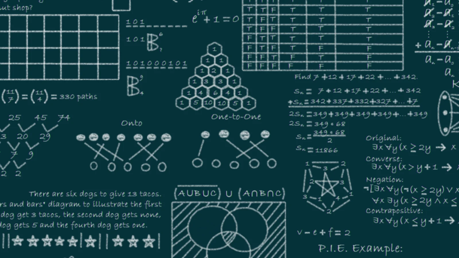
We often find it useful to abbreviate a sum as follows: $$ s=\sum_{i=1}^{n} a_{i}=a_{1}+a_{2}+a_{3}+\cdots+a_{n} $$ We can view this as an algorithm or program: Let s hold the sum at the end, and double [] a be an array holding the numbers we wish to add, that is a [i] $=a_{i}$, then: double $s=0$ for $(i=1 ; i<=n ; i++)$ double $s=0$ for $(i=1 ; i<$ $\quad s=s+a[i]$ $s=s+a[i]$ computes the sum. The most common use of sums for our purposes is when investigating the time complexity of an algorithm or program. For that, we often have to count a variant of $1+2+\cdots+n$, so it is helpful to know that: $$ \sum_{i=1}^{n} i=1+2+\ldots+n=\frac{n(n+1)}{2} $$
In computer science, the obvious way to store an ordered collection of items is as an array. Array items are typically stored in a sequence of computer memory locations, but to discuss them, we need a convenient way to write them down on paper. We can just write the items in order, separated by commas and enclosed by square brackets. Thus, $$ [1,4,17,3,90,79,4,6,81] $$ is an example of an array of integers. If we call this array $a$, we can write it as: $$ a=[1,4,17,3,90,79,4,6,81] $$ This array $a$ has 9 items, and hence we say that its size is 9 . In everyday life, we usually start counting from 1. When we work with arrays in computer science, however, we more often (though not always) start from 0 . Thus, for our array $a$, its positions are $0,1,2, \ldots, 7,8$. The element in the $8^{\text {th }}$ position is 81 , and we use the notation a [8] to denote this element. More generally, for any integer $i$ denoting a position, we write $a[i]$ to denote the element in the $i$ th position. This position $i$ is called an index (and the plural is indices). Then, in the above example, $a[0]=1, a[1]=4, a[2]=17$, and so on.