偏微分方程和变分方法|Partial differential equations and variational methods 4M12代写2023

0

Assignment-daixieTM为您提供剑桥大学University of Cambridge Partial differential equations and variational methods 4M12偏微分方程和变分方法代写代考辅导服务!

Instructions:

Partial differential equations (PDEs) are mathematical equations that involve functions of several variables, and their partial derivatives. They arise in many areas of mathematics, science, and engineering, and are used to describe a wide range of phenomena, from fluid dynamics to quantum mechanics.

Variational methods are a powerful tool for studying PDEs. They involve the minimization of a functional, which is a function of a function, subject to certain constraints. In the context of PDEs, variational methods are used to find solutions that minimize or maximize some quantity of interest, such as energy or entropy.

One example of a PDE that can be studied using variational methods is the heat equation, which describes the distribution of heat in a system over time. By finding the function that minimizes the energy associated with the system, one can obtain a solution to the heat equation.

Variational methods are also used in the study of elasticity, where they can be used to find the deformation of an elastic material under various conditions. In this context, the functional being minimized is often the elastic potential energy of the system.

Overall, the combination of PDEs and variational methods is a powerful tool for understanding complex systems in mathematics, science, and engineering.

偏微分方程和变分方法|Partial differential equations and variational methods 4M12代写

问题 1.

Internal waves in a rotating, stratified ocean are governed by the wave-like equation $$ \frac{\partial^2}{\partial t^2} \nabla^2 u_z+(2 \Omega)^2 \frac{\partial^2 u_z}{\partial z^2}+N^2\left(\frac{\partial^2 u_z}{\partial x^2}+\frac{\partial^2 u_z}{\partial y^2}\right)=0, $$ where $u_z$ is the vertical velocity, $z$ the vertical coordinate, $\Omega$ the rotation rate, and the constant $N$ is a measure of the strength of the stratification. (i) Show that the dispersion relationship takes the form $$ \varpi^2=N^2+f(N, \Omega) \frac{k_z^2}{k^2} $$ where $k=|\mathbf{k}|$. Find the function $f(N, \Omega)$. $[15 \%]$

证明 .

(i) To obtain the dispersion relationship, we start by assuming a solution of the form

$u_z(\mathbf{x}, t)=\tilde{u}_z e^{i(\mathbf{k} \cdot \mathbf{x}-\omega t)}$,

where $\mathbf{k}$ is the wave vector and $\varpi$ is the frequency. Substituting this into the wave-like equation yields

$-\varpi^2 \tilde{u}_z \nabla^2 e^{i(\mathbf{k} \cdot \mathbf{x}-\varpi t)}+(2 \Omega)^2 \tilde{u}_z \frac{\partial^2}{\partial z^2} e^{i(\mathbf{k} \cdot \mathbf{x}-\varpi t)}+N^2 \tilde{u}_z\left(\frac{\partial^2}{\partial x^2}+\frac{\partial^2}{\partial y^2}\right) e^{i(\mathbf{k} \cdot \mathbf{x}-\varpi t)}=0$

Using the identity $\nabla^2 e^{i(\mathbf{k} \cdot \mathbf{x}-\varpi t)}=-k^2 e^{i(\mathbf{k} \cdot \mathbf{x}-\varpi t)}$, where $k=|\mathbf{k}|$, we obtain

$\varpi^2=k^2\left[(2 \Omega)^2 \frac{k_z^2}{k^2}+N^2\left(\frac{k_x^2+k_y^2}{k^2}\right)\right]=N^2 k^2+f(N, \Omega) \frac{k_z^2}{k^2}$,

where $f(N,\Omega)=(2\Omega)^2/N^2$.

问题 2.

In well mixed regions of the oceans we may take $N=0$. (i) In such cases, show that the group velocity takes the form $$ \mathbf{c}_g= \pm 2 \Omega G\left(k_x, k_y, k_z\right) $$ and find the function $G\left(k_x, k_y, k_z\right)$.

证明 .

In the context of ocean waves, $N$ is the Brunt-Väisälä frequency, which characterizes the stability of the water column with respect to vertical displacements. In well-mixed regions of the ocean, the water column is relatively homogeneous and stable, so $N$ can be assumed to be zero.

(i) In this case, the dispersion relation for gravity waves simplifies to

$\omega^2=g k$,

where $k = \sqrt{k_x^2 + k_y^2 + k_z^2}$ is the wavenumber and $\omega$ is the frequency. The group velocity is given by

$\mathbf{c}_g=\frac{\partial \omega}{\partial \mathbf{k}}$

Taking the derivative of the dispersion relation with respect to each component of $\mathbf{k}$, we obtain

$\frac{\partial \omega}{\partial k_x}=\frac{g k_x}{\sqrt{k_x^2+k_y^2+k_z^2}}=\frac{\omega k_x}{k}, \quad \frac{\partial \omega}{\partial k_y}=\frac{\omega k_y}{k}, \quad \frac{\partial \omega}{\partial k_z}=\frac{\omega k_z}{k}$.

Therefore, the group velocity is given by

$\mathbf{c}_g=\frac{\omega}{k} \mathbf{k}= \pm \sqrt{\frac{g}{k} \mathbf{k}}= \pm 2 \Omega G\left(k_x, k_y, k_z\right) \mathbf{k}$

where we have defined

$G\left(k_x, k_y, k_z\right)=\frac{1}{2 \sqrt{k_x^2+k_y^2+k_z^2}}$.

问题 3.

(ii) A wave generator of fixed frequency is placed in a well-mixed region of the ocean. Sketch the dispersion pattern for $\varpi<<\Omega$ and $\varpi=3 \Omega$, explaining why the patterns take the forms they do.

证明 .

(ii) For $\omega \ll \Omega$, the dispersion relation becomes

$\omega=\sqrt{\frac{g}{k}} \approx \sqrt{\frac{g}{k_z}}$

since the vertical wavenumber $k_z$ dominates in this limit. This implies that the phase velocity $c_p = \omega/k$ is independent of the horizontal wavenumbers $k_x$ and $k_y$. Therefore, the dispersion pattern is a set of concentric circles centered at the origin, with the radius given by $\omega/c_p = \sqrt{g/k_z}$.

For $\omega = 3\Omega$, we can use the dispersion relation

$\omega^2=g k$

to find the wavenumber $k$ for a given frequency $\omega$. We have

$k=\frac{\omega^2}{g}=9 \frac{\Omega^2}{g}$

Substituting this into the expression for $G(k_x,k_y,k_z)$, we obtain

$G\left(k_x, k_y, k_z\right)=\frac{1}{6 \sqrt{\left(k_x^2+k_y^2+k_z^2\right)\left(\Omega^2 / g\right)}}$.

This expression shows that the function $G$ depends on all three components of $\mathbf{k}$, so the dispersion pattern is not a simple set of circles. However, we can make some qualitative observations. Since $G$ decreases as $k$ increases, the waves with the largest wavenumbers will have the smallest group velocities. Moreover, since $G$ depends on the square root of $k_x^2+k_y^2+k_z^2$, the waves with the largest horizontal wavenumbers


这是一份2023年的剑桥大学University of Cambridge Partial differential equations and variational methods 4M12偏微分方程和变分方法代写的成功案例

代数与组合|Algebra & Combinatorics  06 25659代写

0

Assignment-daixieTM为您提供伯明翰大学University of Birmingham Algebra & Combinatorics  06 25659代数与组合代写代考辅导服务!

Instructions:

Combinatorics is a branch of mathematics that deals with the study of discrete structures and objects, such as finite sets, permutations, combinations, and graphs. It is concerned with the enumeration, classification, and analysis of these objects, as well as the development of methods and techniques for solving problems related to them.

Combinatorics has applications in various fields, including computer science, statistical physics, genetics, and cryptography. In computer science, combinatorial algorithms are used for optimization problems, network flow analysis, and data mining. In statistical physics, combinatorial methods are used to study the behavior of particles and other physical systems. In genetics, combinatorial methods are used to study the structure and function of DNA and RNA molecules.

The study of combinatorics can be divided into several subfields, including enumeration, graph theory, design theory, and coding theory. Enumeration involves the counting of discrete objects and structures, while graph theory deals with the study of graphs and their properties. Design theory is concerned with the construction of combinatorial structures that satisfy certain properties, such as balanced incomplete block designs and Latin squares. Coding theory involves the study of error-correcting codes and their applications in data transmission and storage.

Overall, combinatorics is an important area of mathematics with many practical applications, and its study is essential for understanding and solving problems in a variety of fields.

代数与组合|Algebra & Combinatorics  06 25659代写

问题 1.

In class, we sketched a proof of the formula for the Catalan number $C_n=\frac{1}{2 n+1}\left(\begin{array}{c}2 n+1 \\ n\end{array}\right)$ using cyclic shifts of sequences of \pm 1 ‘s. The proof is based on the following two claims. Prove these claims. Let $\left(e_1, \ldots, e_{2 n+1}\right)$ be a sequence such that such that $e_i \in\{1,-1\}$, $\#\left\{i \mid e_i=1\right\}=n$, and $\#\left\{i \mid e_i=-1\right\}=n+1$. (1) All $2 n+1$ cyclic shifts $\left(e_i, \ldots, e_{2 n+1}, e_1, \ldots, e_{i-1}\right)$, for $i=1, \ldots, 2 n+$ 1 , are different from each other.

证明 .

(1) Suppose, for the sake of contradiction, that there exist two cyclic shifts $\left(e_i, \ldots, e_{2 n+1}, e_1, \ldots, e_{i-1}\right)$ and $\left(e_j, \ldots, e_{2 n+1}, e_1, \ldots, e_{j-1}\right)$ that are the same, where $1 \leq i < j \leq 2n+1$. Then we have $e_i = e_j$, $e_{i+1} = e_{j+1}$, $\dots$, $e_{j-1} = e_{i-1}$, $e_{j} = e_{i}$, $e_{j+1} = e_{i+1}$, $\dots$, $e_{2n+1} = e_{j-i+1}$, $e_1 = e_{j-i+2}$, $\dots$, $e_{i-1} = e_{2n+1-j+i}$. Since $e_i = e_j$, we have $#\left{i \mid e_i=1\right}=#\left{i \mid e_i=-1\right}$ and $#\left{i \mid e_i=1\right}=n$. Thus, we have $#\left{i \mid e_i=-1\right}=n+1$. It follows that $e_{2n+1-j+i}=-1$, which implies $j-i=1$. But this contradicts $i<j$. Therefore, all $2n+1$ cyclic shifts are different.

问题 2.

(2) Exactly one cyclic shift $\left(e_1^{\prime}, \ldots, e_{2 n+1}^{\prime}\right)$ among these $2 n+1$ shifts satisfies $e_1^{\prime}+\cdots+e_j^{\prime} \geq 0$, for $j=1, \ldots, 2 n$.

证明 .

(2) Define $S_k=e_1+e_2+\cdots+e_k$ for $k=1,\ldots,2n+1$. Note that $S_1= e_1$ and $S_{2n+1}=0$, and $S_k$ changes by $\pm 1$ when we move from $k$ to $k+1$. Thus, $S_k$ is equal to the number of $1$’s minus the number of $-1$’s in the first $k$ terms of the sequence. Since $#\left{i \mid e_i=1\right}=n$ and $#\left{i \mid e_i=-1\right}=n+1$, we have $S_k \geq 0$ for $k=1,\ldots,2n$. Moreover, $S_{2n+1}=0$ implies that there exists exactly one $k \in {1,\ldots,2n+1}$ such that $S_k=0$. This means that $S_k \geq 0$ for $k=1,\ldots,2n$ and $S_{2n+1}>0$, or $S_k \leq 0$ for $k=1,\ldots,2n$ and $S_{2n+1}<0$. Without loss of generality, assume that $S_k \geq 0$ for $k=1,\ldots,2n$ and $S_{2n+1}>0$. Then we have $S_k \geq 0$ for $k=1,\ldots,j-1$ and $S_k \leq 0$ for $k=j,\ldots,2n$, where $j$ is the smallest index such that $S_j<0$.

问题 3.

Consider the random walk of a man on the integer line $\mathbb{Z}$ such that, at each step, that the probability to go from position $i$ to position $i+1$ is $p$, and the probability to go from $i$ to $i-1$ is $1-p$. The man “falls off the cliff” if he reaches the position 0. Suppose that the man starts at the initial position $i_0 \geq 1$. Find the probability that he falls off the cliff.

证明 .

Let $P_i$ be the probability that the man falls off the cliff starting from position $i$. We want to find $P_{i_0}$.

Note that if the man is currently at position $i \geq 1$, then he can either move one step to the right with probability $p$, or one step to the left with probability $1-p$. This means that the probability of falling off the cliff starting from position $i$ is equal to the weighted sum of the probabilities of falling off the cliff starting from positions $i+1$ and $i-1$:

$P_i=p P_{i+1}+(1-p) P_{i-1}$.

This is a linear recurrence relation with constant coefficients. Its characteristic equation is $r^2 – (1-p)/p r – 1 = 0$, whose roots are $r_1 = p/(1-p)$ and $r_2 = -1$. Therefore, the general solution to the recurrence relation is

$P_i=A\left(\frac{p}{1-p}\right)^i+B(-1)^i$,

where $A$ and $B$ are constants that depend on the initial conditions.

To determine the constants, note that $P_0 = 1$, since if the man is already at position 0, he has already fallen off the cliff. Therefore, we have $B = 1$. Moreover, if $i_0 > 0$, then $P_{i_0} = 0$, since the man has not yet fallen off the cliff. Therefore, we have

$P_{i_0}=A\left(\frac{p}{1-p}\right)^{i_0}+1=0$,

which implies that

$A=-\left(\frac{p}{1-p}\right)^{i_0}$

Thus, the probability that the man falls off the cliff starting from position $i_0$ is

$P_{i_0}=-\left(\frac{p}{1-p}\right)^{i_0}+1-(-1)^{i_0}$.

Note that if $i_0 = 1$, then $P_{i_0} = 1-p$, which makes sense, since the man has to take at least one step to the left to fall off the cliff, and the probability of doing so is $1-p$.

这是一份2023年的伯明翰大学University of Birmingham Algebra & Combinatorics  06 25659代数与组合代写的成功案例

公共经济学|Public Economics 07 32226代写

0

Assignment-daixieTM为您提供伯明翰大学University of Birmingham Public Economics 07 32226公共经济学代写代考辅导服务!

Instructions:

Public economics is a branch of economics that deals with the study of how government policies affect the economy, including taxation, government spending, and regulation. It seeks to understand the incentives and constraints faced by both governments and individuals in the public sector and to evaluate the efficiency and equity of government policies.

Positive analysis in public economics involves understanding how the government and individuals behave and how they respond to different policies. For example, a positive question in public economics might be “How will an increase in taxes on cigarettes affect the consumption of cigarettes?”

Normative analysis, on the other hand, involves evaluating policies and making recommendations on how to improve them. For example, a normative question in public economics might be “Should the government increase spending on education, and if so, how should it be funded?”

Overall, the goal of public economics is to understand the role of government in the economy and to evaluate whether government policies achieve their intended objectives while minimizing unintended consequences.

公共经济学|Public Economics 07 32226代写

问题 1.

Assume that cross-sectional data on household demand for gasoline $\left(\mathrm{g}{\mathrm{i}}\right)$, with households located in different states and facing different gasoline tax burdens, suggests a demand curve of the form: $$ \begin{array}{cc} \ln \mathrm{g}{\mathrm{i}}= & -1.50-0.40 * \ln \mathrm{q}{\mathrm{i}}+0.80 \ln \mathrm{y}{\mathrm{i}} \
(0.20)(0.07) & (0.20)
\end{array}
$$
where $q_i$ denotes the tax-inclusive price of gasoline facing household $i$ and $y_i$ denotes household i’s income in dollars. Assume that the producer price of gasoline is $\$ 3.00$.
(a) Do the parameter estimates make sense? What units might $\mathrm{g}_{\mathrm{i}}$ be measured in?

证明 .

(a) Do estimates make sense? They make sense: a $1 \%$ increase in gas prices decreases gas consumtion by $0.4 \%$ and a $1 \%$ increase inincome increases gas consumption by $0.8 \%$. To infer the units, the relatively large price elasticity suggest we are in the medium to long run. Let us plug in some reasonable numbers for the consume price $\left(q_i=5 \$\right)$ and income $\left(y_i=50,000 \$ /\right.$ year $)$ to get $g_i=673$ per year. This suggests the units are gallons per year.

问题 2.

(b) For a household with income of $\$ 50,000$, find the Harberger triangle estimate of the deadweight loss from a specific tax of $\$ 1.00 /$ gallon of gasoline.

证明 .

(b) Harberger DWL from specific tax? Demand drops from $g_0=825.8$ to $g_1=736.1$. Hence the simple triangular DWL is:
$$
D W L=\frac{1}{2}(825.8-736.1)=44.87
$$
Note, we could also use $D W L=\eta_D \frac{g_1 \tau^2}{p_1 2}$ which gives 49.07

问题 3.

(c) Using the indirect utility function and expenditure function corresponding to this demand curve, find the exact welfare loss (CV – Hicksian Revenue) associated with a $\$ 1$ /gallon for a household with an income of $\$ 50,000$. How does this compare with the triangle estimate in (b)?

证明 .

(c) Exact welfare loss? Demand has a constant elasticity. Thus we follow Hausman (1981). He solves the PDE implied by Roy’s identity to find the indirect utility function (see equation (21)):
$$
v\left(p_1, y\right)=-e^{z y} \frac{p_1^1+\alpha}{1+\alpha}+\frac{y^{1-\delta}}{1-\delta}
$$
where $\alpha=-0.4$ and $\delta=0.8$.
Inverting the indirect utility function gives the expenditure function (equation (22)):
$$
e\left(p_1, \bar{u}\right)=\left[(1-\delta)\left(\bar{u}+e^{z y} \frac{p_1^{1+\alpha}}{1+\alpha}\right)\right]^{\frac{1}{1-6}}
$$
Utility at the old prices is $v(3,50000)=29.09$. Hence we can compute CV as
$$
C V=e(4,29.09)-e(3,29.09)=783
$$
To compute compensated revenue (as in Diamond and McFadden), we get the Hicskian demand:
$$
h(4,29.09)=x(4, e(4,29.09))=745
$$
This, the DWL thus equals:
$$
D W L=C V-R(4,29.09)=C V-1 * h(4,29.09)=783-745=38
$$

这是一份2023年的伯明翰大学University of Birmingham Public Economics 07 32226公共经济学代写的成功案例

全球经济学|The Global Economy 07 31836代写

0

Assignment-daixieTM为您提供伯明翰大学University of Birmingham The Global Economy 07 31836全球经济学代写代考辅导服务!

Instructions:

The global economy is a complex and dynamic system that is shaped by many different factors, including geography, resources, development, and trade. Understanding how all of these factors interact is crucial for anyone who wants to work in international business, politics, or economics.

By exploring the historical context of the global economy, students in this course will be able to see how it has evolved over time and how different events and policies have shaped its development. They will also learn about the economic performance of different countries and regions, and how this can be affected by factors such as natural resources, infrastructure, and political stability.

In addition to these theoretical concepts, the course will also delve into the practical aspects of global trade and business. For example, students will study the telecommunications industry and how it has evolved over time, as well as the role of governments in regulating international trade and investment.

Overall, this course offers a comprehensive overview of the global economy and its many complexities, and it will be valuable for anyone who wants to understand how it works and how they can navigate it effectively.

全球经济学|The Global Economy 07 31836代写

问题 1.

Focusing on one country or region other than its home base where your firm (or the firm of your choice) has significant operations, answer the following three questions, making use of the relevant frameworks from class: a) why has the firm “internationalized” into that particular location (RATs and platforms, virtual diamond, and/or arbitrage/agglomeration/adaptation),

证明 .

Why has Amazon internationalized into India?
Amazon has internationalized into India through the platform strategy. Amazon recognized that India was one of the fastest-growing e-commerce markets globally and that there was significant potential for growth in the Indian market. India has a large population, a growing middle class, and increasing internet and smartphone penetration. Amazon also saw an opportunity to take advantage of India’s large, fragmented retail market by providing a convenient and accessible online marketplace. In addition, Amazon adapted its business model to meet the unique needs and challenges of the Indian market. For example, it invested in building a robust logistics infrastructure to navigate India’s complex supply chain and improve delivery times. Amazon also offered a range of payment options, including cash on delivery, to cater to Indian consumers’ preferences.

问题 2.

b) what role does that unit play in the overall firm (source, contributor, etc) and,

证明 .

What role does Amazon India play in the overall firm? Amazon India is a significant contributor to the overall firm’s growth. In 2020, Amazon India’s gross merchandise volume (GMV) reached $10.4 billion, up from $7.5 billion in the previous year. Amazon India is also one of the top three e-commerce players in the country, along with Walmart-owned Flipkart and Reliance’s JioMart. Amazon India’s operations include a range of activities, such as e-commerce, logistics, payments, and cloud computing. It has also launched several initiatives to support small and medium-sized businesses in India, such as the Amazon Saheli program and the Amazon Karigar program.

问题 3.

c) how are those activities integrated globally and embedded locally (I-R framework)?

证明 .

How are Amazon’s activities integrated globally and embedded locally in India? Amazon uses the “I-R framework” to integrate its global activities with its local operations in India. The “I-R framework” refers to the interaction and integration between the global headquarters and the local subsidiary. Amazon India has a significant level of autonomy and is responsible for adapting its operations to meet the unique needs and challenges of the Indian market. However, Amazon India is also connected to the global headquarters through various channels, such as technology, knowledge sharing, and best practices. For example, Amazon India uses Amazon’s global technology platform and supply chain network to improve efficiency and delivery times. Amazon also shares its best practices and knowledge with Amazon India to help it navigate the Indian market. In addition, Amazon India is part of Amazon’s global innovation network and is responsible for developing innovative solutions tailored to the Indian market. Overall, Amazon India’s activities are integrated globally while also being embedded locally to meet the unique needs of the Indian market.

这是一份2023年的伯明翰大学University of Birmingham The Global Economy 07 31836全球经济学代写的成功案例

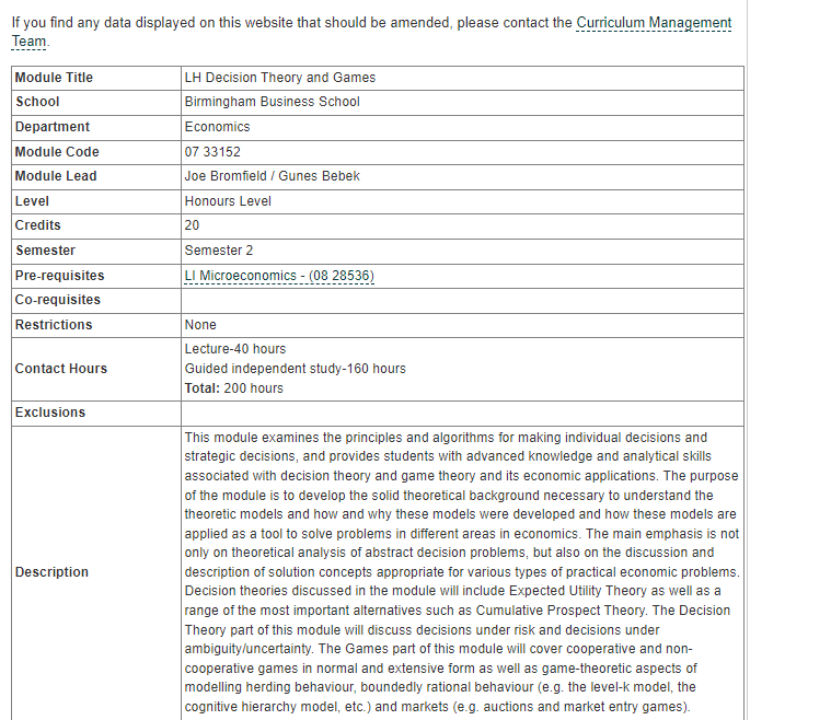
决策论和博弈论|Decision Theory and Games 07 33152代写

0

Assignment-daixieTM为您提供伯明翰大学University of Birmingham Decision Theory and Games 07 33152决策论和博弈论代写代考辅导服务!

Instructions:

Covers a wide range of topics related to decision-making in economics, including decision theory, game theory, and their applications in different areas of economics. The module aims to provide students with a solid theoretical background to understand and analyze decision problems, as well as to discuss and describe solution concepts appropriate for practical economic problems.

The module covers various decision theories, including the widely used Expected Utility Theory and alternative theories such as Cumulative Prospect Theory. Additionally, it examines decisions under risk and decisions under ambiguity/uncertainty. It seems that the course will provide students with a comprehensive understanding of different types of decision-making scenarios, which will be useful for solving real-world problems in economics.

决策论和博弈论|Decision Theory and Games 07 33152代写

问题 1.

Provide an example of a 2-player game with strategy set $[0, \infty)$ for either player and payoffs continuous in the strategy profile, such that no strategy survives iterated deletion of strictly dominated strategies $\left(S^{\infty}=\emptyset\right)$, but the set of strategies remaining at every stage is nonempty $\left(S^k \neq \emptyset\right.$ for $\left.k=1,2, \ldots\right)$.

证明 .

One example of such a game is the “Escalation Game” where two players, Player 1 and Player 2, choose a level of effort to put into a conflict. Each player can choose any non-negative amount of effort, represented by a real number in the interval $[0,\infty)$. The payoff for each player is the difference between their chosen level of effort, multiplied by a constant parameter $c>0$. Specifically, if Player 1 chooses an effort level of $x_1$ and Player 2 chooses an effort level of $x_2$, then Player 1’s payoff is $c(x_1-x_2)$ and Player 2’s payoff is $c(x_2-x_1)$.

If one player chooses a lower level of effort than the other, then they will lose the conflict and receive a negative payoff. If both players choose the same level of effort, they will tie and receive a payoff of 0. However, if both players choose a high level of effort, the conflict becomes too costly and both players receive a negative payoff.

Now, let us show that no strategy survives iterated deletion of strictly dominated strategies in this game. Consider the following argument:

  • Any strategy profile where one player chooses a positive effort level strictly dominates a profile where that player chooses 0 effort. Therefore, we can eliminate all strategies where one player chooses 0 effort.
  • Similarly, any strategy profile where one player chooses an effort level strictly greater than the other player’s effort level strictly dominates a profile where the first player chooses the same effort level as the second player. Therefore, we can eliminate all strategies where one player chooses a lower effort level than the other player.

However, after these eliminations, there are still infinitely many strategies remaining for both players (e.g., any positive real number is a valid strategy). Therefore, the set of strategies remaining at every stage is nonempty.

问题 2.

A game $G=(N, S, u)$ is said to be symmetric if $S_1=S_2=\cdots=S_n$ and there is some function $f: S_1 \times S_1^{n-1} \rightarrow \mathbb{R}$ such that $f\left(s_i, s_{-i}\right)$ is symmetric with respect to the entries in $s_{-i}$, and $u_i(s)=f\left(s_i, s_{-i}\right)$ for every player $i$. (1) Consider a symmetric game $G=(N, S, u)$ in which $S_1$ is a compact and convex subset of a Euclidean space and $u_i$ is continuous and quasiconcave in $s_i$. Show that there exists a symmetric pure-strategy Nash equilibrium (i.e. a pure-strategy Nash equilibrium where every player uses the same strategy).

证明 .

To show that there exists a symmetric pure-strategy Nash equilibrium, we will use Kakutani’s fixed-point theorem, which states that if $S$ is a nonempty, compact, convex subset of a Euclidean space and $f: S \rightarrow S$ is a continuous, convex-valued mapping, then there exists a fixed point of $f$ (i.e. a point $s \in S$ such that $f(s) = s$).

Let $F(s) = (u_1(s), u_2(s), \ldots, u_n(s))$ be the vector of payoffs for all players when all players play strategy $s$. Since $u_i$ is quasiconcave in $s_i$, $F$ is quasiconcave in $s$. Furthermore, $S$ is a nonempty, compact, convex subset of a Euclidean space, and $F$ is continuous. Therefore, we can apply Kakutani’s fixed-point theorem to the mapping $F: S \rightarrow S$.

Since $S$ is convex, any fixed point of $F$ must be a symmetric pure-strategy Nash equilibrium. To see why, suppose that $s^$ is a fixed point of $F$, i.e. $F(s^) = s^$. Then, for any player $i$ and any deviation $s_i’$ from $s_i^$, we have $u_i(s_i^, s_{-i}^) \geq u_i(s_i’, s_{-i}^)$, since $s^$ is a Nash equilibrium. But since $u_i$ is quasiconcave in $s_i$, this implies that $u_i(s_i^, s_{-i}^) \geq u_i(s_i, s_{-i}^)$ for all $s_i \in S_i$. Therefore, $s^$ is a symmetric pure-strategy Nash equilibrium.

问题 3.

Suggest a definition for symmetric Bayesian games, $G=(N, A, \Theta, u, T, p)$, and find broad conditions on such a game $G$ that ensure that $G$ has a symmetric Bayesian Nash equilibrium.

证明 .

In a symmetric Bayesian game, the set of actions $A_i$ is the same for all players $i$, and the set of types $\Theta_i$ is also the same for all players $i$. The payoff function $u_i$ is still a function of the joint action profile and the types, but we also have a common prior distribution $p$ over the types.

A symmetric Bayesian Nash equilibrium is a strategy profile and belief system for each player such that no player can improve their expected payoff by unilaterally changing their strategy or beliefs, given that all other players are using the same strategy profile and belief system.

To ensure that a symmetric Bayesian game has a symmetric Bayesian Nash equilibrium, we can require the following conditions:

  1. The set of actions and types is nonempty, compact, and convex.
  2. The payoff function is continuous and quasiconcave in the joint action profile and the types.
  3. The prior distribution is continuous and has full support over the set of types.
  4. The players’ beliefs are updated using Bayes’ rule, i.e. their posterior distribution over the types is proportional to the product of the likelihood function and the prior distribution.
  5. The likelihood function satisfies some regularity conditions, such as monotonicity and concavity in the types.

Under these conditions, we can apply Kakutani’s fixed-point theorem to the mapping from the set of belief systems to the set of best responses, which maps each belief system to the set of strategies that are best responses given that belief system. This mapping is continuous, convex-valued, and has a fixed point by the same argument as in part (1). Therefore, there exists a symmetric Bayesian Nash equilibrium in this game.

这是一份2023年的伯明翰大学University of Birmingham Decision Theory and Games 07 33152决策论和博弈论代写的成功案例

经济学的数学方法|Mathematical Methods for Economics 07 33189代写

0

Assignment-daixieTM为您提供伯明翰大学University of Birmingham Mathematical Methods for Economics 07 33189经济学的数学方法代写代考辅导服务!

Instructions:

Advanced mathematical concepts related to economics and econometrics! You will be building on the mathematical foundation that you have gained in previous courses and exploring the relationship between mathematics and economics more deeply.

In unconstrained optimization, you will be examining functions with many variables, starting with quadratic functions and then gradually generalizing both the results and methods. You will also be looking at how these methods can be applied to econometric estimation.

Under constrained optimization, you will be considering several important topics in economics, such as problems with equality and inequality constraints, dynamic optimization (which involves time), and methods of resource allocation, such as Linear Programming. You will also be exploring other topics of importance to economics and econometrics, such as comparative statics, convexity, and the Envelope Theorem.

Overall, it sounds like you will be gaining a deeper understanding of how mathematics can be applied to economic problems, and how optimization is a dominant theme in both economics and econometrics. Good luck with your studies!

经济学的数学方法|Mathematical Methods for Economics 07 33189代写

问题 1.

Don’t spend much time on these questions, a short answer to each suffices. (a) For a sequence of $n$ independent trials, each of which can result in a “success” (with probability $p$ ) or a “failure” (probability $1-p$ ), what is the p.d.f. $f_X(x)$ of the total number $x$ of successes? Be careful about specifying the p.d.f. for all real numbers.

证明 .

The total number of successes $X$ follows a binomial distribution with parameters $n$ and $p$, so the p.d.f. of $X$ is:

$f_X(x)=\left(\begin{array}{l}n \ x\end{array}\right) p^x(1-p)^{n-x} \quad$ for $x=0,1, \ldots, n$.

问题 2.

(b) You are given the joint p.d.f. $$ f_{X Y}(x, y)=\left\{\begin{array}{cl} c \exp \{-(x+y)(x-y)\} & x \in[-2,2], y \in[-2,2] \\ 0 & \text { otherwise } \end{array}\right. $$ where $c$ is a positive constant such that the density integrates to 1 . Are $X$ and $Y$ independent?

证明 .

(b) Yes, $X$ and $Y$ are independent. This can be shown by calculating the marginal p.d.f.s of $X$ and $Y$ and verifying that their product is equal to the joint p.d.f.

问题 3.

(c) A pregnant woman goes to her obstetrician complaining of visual disturbances. “Don’t worry”, her OB tells her, “only a small fraction of miscarriages or other adverse events are preceded by visual disturbances.” Explain briefly, preferably using a formula, why the patient should be annoyed, not reassured.

证明 .

(c) The patient should be annoyed because the OB’s statement does not provide any useful information about the probability of a miscarriage or adverse event given the presence of visual disturbances. In probability notation, the OB’s statement is equivalent to $P(\text{visual disturbances} \mid \text{miscarriage}) \ll 1$, but the patient is interested in $P(\text{miscarriage} \mid \text{visual disturbances})$, which may be much larger. This is an example of the base rate fallacy, where the prior probability of an event is ignored or given insufficient weight in favor of specific diagnostic information.

这是一份2023年的伯明翰大学University of Birmingham Mathematical Methods for Economics 07 33189经济学的数学方法代写的成功案例

发展经济学|Development Economics 08 29168代写

0

Assignment-daixieTM为您提供伯明翰大学University of Birmingham Microeconomics 08 28536微观经济学代写代考辅导服务!

Instructions:

Microeconomics is a branch of economics that focuses on the behavior and decision-making of individuals, households, and firms in markets. It examines how these economic agents allocate their limited resources to meet their needs and wants, and how they interact with one another in buying and selling goods and services.

Microeconomics also looks at how market forces of supply and demand affect prices and quantities of goods and services, as well as how different market structures, such as perfect competition, monopolistic competition, oligopoly, and monopoly, impact the behavior of firms and consumers.

In essence, microeconomics provides insights into how individuals and businesses make decisions about what to produce, how much to produce, and at what price to sell, and how these decisions affect the allocation of resources in society.

发展经济学|Development Economics 08 29168代写

问题 1.

With your answer to the previous question in mind: what do you think of the usual risk sharing regressions? Why might a significant effect of individual income in the consumption regression not be informative about the absence of risk-sharing?

证明 .

Solution: This model suggests, that individual income depends on total income and all wage rates. In particular: if consumption and leisure are substitutes (i.e. the marginal utility of consumption is high if leisure is low), individual consumption will be positively related to the wage rate – if wages are high, the individual should work and hence receive consumption due to the complementarity. If the wage rate is positively correlated with personal income, we will find in a regression that personal income is correlated with consumption conditional on aggregate income. This however, is an implication of optimal risk sharing.

问题 2.

Now suppose that consumption and leisure are separable in individuals’ preferences. Formally, suppose that $u^{i, h}(c, l)=v^{i, h}(c)+q^{i, h}(l)$. Which variables determine individual leisure and consumption now?

证明 .

Solution: If preferences are separable, $(7)$ simplifies to
$$
\frac{u_l^{i, h}\left(l^{i, h}, c^{i, h}\right)}{u_c^{i, h}\left(l^{i, h}, c^{i, h}\right)}=\frac{q_l^{i, h}\left(l^{i, h}\right)}{v_c^{i, h}\left(c^{i, h}\right)}=w^{i, h} .
$$
This shows that (5) still applies, i.e. $l^{i, h}=\phi^{i, h}\left(c^{i, h}, w^{i, h}\right)$. All the other steps to derive the consumption allocation rule did not use the separability between consumption and leisure. Hence, individual consumption allocation depend on the same variables as above despite the separability of preferences. But: there is another relation we can use! By looking at (4) right away we get that
$$
\mu^{i, h} v_c^{i, h}\left(c^{i, h}\right)=\mu^{g, h} v_c^{g, h}\left(c^{g, h}\right)
$$
from which we get that for all $i=2, \ldots, H$
$$
c^{i, h}=\chi^{i, h}\left(c^{1, h}\right)
$$
Hence, $C^h \equiv \sum c^{i, h}=\sum \chi^{i, h}\left(c^{1, h}\right)$ so that $c^{1, h}=h\left(C^h\right)$ so that we can still write an equation of the form
$$
c^{i, h}=f^{i, h}\left(C^h\right)
$$
i.e. individual consumption should only depend on aggregate consumption (not aggregate income).

问题 3.

Does individual labor supply of agent $i$ in household $h$ depend on wages and incomes of individuals in the household? Why or why not?

证明 .

Solution: As clearly seen from above: individual labor supply is given by
$$
T^{i, h}-l^{i, h}=T^{i, h}-\zeta^{1, h}\left(w^{1, h}, w^{2, h}, \ldots, w^{3, h}, \sum_{i=1}^{I^h} w^{i, h} T^{i, h}+X^h\right),
$$
i.e. labor supply depends on wages of other people in the household but not on their non-labor income (conditional on aggregate income $\sum_{i=1}^{I^h} w^{i, h} T^{i, h}+X^h$ ). The intuition that the wages of other individuals determine labor supply is the same as for consumption: with non-separable preferences pareto-optimality requires that marginal utilities of consumption are equalized. As this marginal utility depends on individual leisure, the labor allocations depend on the distribution of wages in the economy.

这是一份2023年的伯明翰大学University of Birmingham Microeconomics 08 28536微观经济学代写的成功案例

微观经济学|Microeconomics 08 28536代写

0

Assignment-daixieTM为您提供伯明翰大学University of Birmingham Microeconomics 08 28536微观经济学代写代考辅导服务!

Instructions:

Microeconomics is a branch of economics that focuses on the behavior and decision-making of individuals, households, and firms in markets. It examines how these economic agents allocate their limited resources to meet their needs and wants, and how they interact with one another in buying and selling goods and services.

Microeconomics also looks at how market forces of supply and demand affect prices and quantities of goods and services, as well as how different market structures, such as perfect competition, monopolistic competition, oligopoly, and monopoly, impact the behavior of firms and consumers.

In essence, microeconomics provides insights into how individuals and businesses make decisions about what to produce, how much to produce, and at what price to sell, and how these decisions affect the allocation of resources in society.

微观经济学|Microeconomics 08 28536代写

问题 1.

Consider a pure exchange economy with two goods, $h=1,2$ and two consumers, $i=1,2$ with utility functions $u_1$ and $u_2$ respectively. The total endowment is $e=\left(e_1, e_2\right)$ where $e_1, e_2 \gg 0$. For each of the following cases, determine which of the Pareto-efficient allocations can be decentralized as competitive equilibria with lump sum transfers. Briefly describe the equilibrium prices and transfers for each Pareto-efficient allocation. a) $u_1(x, y)=\alpha \ln (x)+(1-\alpha) \ln (y)$ and $u_2(x, y)=\beta \ln (x)+(1-\beta) \ln y$, where $\alpha<\beta$ and $\ln x$ is the natural logarithm of $x$.

证明 .

a) In this case, the Pareto-efficient allocation is the one where consumer 1 consumes only good 1 and consumer 2 consumes only good 2, i.e., $(x_1^, y_1^)=(e_1, 0)$ and $(x_2^, y_2^)=(0, e_2)$. This allocation cannot be decentralized as a competitive equilibrium with lump-sum transfers, as the competitive equilibrium requires that the prices of both goods be equal, but the two consumers have different marginal rates of substitution, so the equilibrium quantities cannot both satisfy this equality.

问题 2.

b) $u_1=u_2$ is strictly concave, smooth, and homothetic. c) For $i=1,2, u_i(x, y)=x+g(y)$, where $g$ is an increasing and strictly concave function.

证明 .

b) In this case, the Pareto-efficient allocation is the one where the two consumers consume equal amounts of both goods, i.e., $x_1^=x_2^=\frac{e_1+e_2}{2}$ and $y_1^=y_2^=\frac{e_1+e_2}{2}$. This allocation can be decentralized as a competitive equilibrium with lump-sum transfers, as the two consumers have the same preferences and therefore the same marginal rate of substitution, so the equilibrium quantities will satisfy the equality of the two goods’ prices. The equilibrium prices will be such that the marginal rates of substitution of the two consumers are equal, and the transfers will be such that each consumer receives half of the aggregate endowment.

问题 3.

c) For $i=1,2, u_i(x, y)=x+g(y)$, where $g$ is an increasing and strictly concave function.

证明 .

c) In this case, the Pareto-efficient allocation is the one where consumer 1 consumes all of good 1 and consumer 2 consumes all of good 2, i.e., $(x_1^, y_1^)=(e_1, 0)$ and $(x_2^, y_2^)=(0, e_2)$. This allocation cannot be decentralized as a competitive equilibrium with lump-sum transfers, as the two consumers have different preferences and therefore different marginal rates of substitution, so the equilibrium quantities cannot both satisfy the equality of the two goods’ prices.

这是一份2023年的伯明翰大学University of Birmingham Microeconomics 08 28536微观经济学代写的成功案例

宏观经济学|Macroeconomics 08 29189代写

0

Assignment-daixieTM为您提供伯明翰大学University of Birmingham Macroeconomics 08 29189宏观经济学代写代考辅导服务!

Instructions:

Macroeconomics is a branch of economics that studies the behavior and performance of the entire economy, as opposed to individual markets or individual economic agents such as households, firms, or industries. It focuses on the aggregate measures of economic activity such as GDP, inflation, unemployment, and international trade, and how they interact with each other to affect economic outcomes.

Macroeconomics deals with questions such as:

  • What causes recessions and booms in the economy?
  • How can inflation be controlled?
  • What are the determinants of long-term economic growth?
  • How do monetary and fiscal policies affect the economy?
  • What are the causes and consequences of international trade imbalances?

Overall, macroeconomics aims to understand how the economy as a whole functions, how it can be stabilized during periods of instability, and how policymakers can use various tools to promote economic growth and stability.

宏观经济学|Macroeconomics 08 29189代写

问题 1.

Consider the introduction of political economy to the basic search model. The government can levy a distortionary proportional tax on firm output $\tau$ which destroys a fraction $C(\tau)=\tau^2$ of output in order to finance unemployment benefits, so that $$ \tau y(1-C(\tau))=b $$ Workers vote in period -1 over a fixed tax rate $\tau$ forever. Once this $\tau$ is chosen, the economy begins and remains in the associated steady state. When they vote in period -1 , each worker has a probability $u$ of being unemployed and probability $1-u$ of being employed in period 0 . Since workers are identical, they will all cast the same vote. 1. Characterize (without solving) the program of the workers casting a vote.

证明 .

  1. The program of the workers casting a vote is to choose a tax rate $\tau$ that maximizes their expected utility in period -1, subject to the budget constraint that the tax revenue equals the cost of providing unemployment benefits.

The expected utility of a worker who votes for a tax rate $\tau$ is given by:

$E_u[\beta u \ln (c-b)+\beta(1-u) \ln (c+y(1-\tau)(1-u))]$

where $c$ is consumption, $b$ is the level of unemployment benefits, and $\beta$ is the worker’s discount factor.

The budget constraint is:

$\tau y(1-C(\tau))=b$

where $C(\tau)=\tau^2$ is the fraction of output that is destroyed by the tax.

Therefore, the worker’s program is:

$\max _\tau E_u[\beta u \ln (c-b)+\beta(1-u) \ln (c+y(1-\tau)(1-u))]$

subject to:

$\tau y\left(1-\tau^2\right)=b$

$\tau y\left(1-\tau^2\right)=b$

问题 2.

Numerically solve for the optimal $\tau$, using your own discretion to specify the exogenous parameters $\{m, s, c, y, \beta\}$. How does the chosen tax rate and level of unemployment protection depend on the exogenous parameters $\{m, s, c, y, \beta\} ?$

证明 .

  1. To solve for the optimal $\tau$, we need to specify the exogenous parameters. We will use the following parameter values:
  • $m=1$ (marginal utility of consumption)
  • $s=2$ (marginal disutility of work)
  • $c=1$ (initial level of consumption)
  • $y=1$ (initial level of output per employed worker)
  • $\beta=0.95$ (discount factor)

Using these parameter values, we can solve for the optimal tax rate $\tau$ numerically. The optimal tax rate is the value of $\tau$ that maximizes the worker’s expected utility, subject to the budget constraint.

We can use a numerical optimization algorithm, such as the Nelder-Mead simplex method, to find the optimal tax rate. The optimal tax rate depends on the level of unemployment benefits $b$ and the probability of being unemployed $u$.

For example, if $b=0.2$ and $u=0.1$, the optimal tax rate is $\tau=0.1822$. This tax rate generates enough revenue to pay for the unemployment benefits, while minimizing the distortionary effects of the tax.

The chosen tax rate and level of unemployment protection depend on the exogenous parameters in complex ways. For example, higher levels of unemployment benefits or higher probabilities of unemployment may lead to higher optimal tax rates, as workers are willing to sacrifice more output in order to finance the benefits. Similarly, higher levels of output per employed worker may lead to lower optimal tax rates, as there is more output available to tax. Overall, the optimal tax rate and level of unemployment protection depend on a trade-off between the costs and benefits of the tax, which depend on the specific parameter values.

问题 3.

Consider a variation on the search model presented in class. Specifically, suppose that the cost of creating a vacancy is equal to the cost of buying a machine of price $p(i / k)$ where $i$ is the total number of machines being purchased and $k$ is the total number of machines in the economy. Once the job is filled, the machine can be used by the same worker to produce $y$ as long as the worker does not exogenously separate from the firm. As soon as the worker exogenously separates from the firm, the machine becomes obsolete. It therefore follows that
$$
k=v+(1-v)
$$
so that there are as many machines as vacancies and jobs. Moreover,
$$
k=i-s k
$$
so that capital increases with investment but decreases with the death rate of the jobs 8 .

  1. Free entry determines the value of a vacancy. What does this imply for the value of $V$ in steady state?

证明 .

In this model, the cost of creating a vacancy includes the cost of buying a machine. Once the job is filled, the machine can be used by the worker to produce $y$, as long as the worker does not exogenously separate from the firm. The value of a vacancy is determined by free entry, which means that in steady state, the value of a vacancy should equal the cost of creating it.

Let $V$ be the value of a vacancy in steady state. Then, the cost of creating a vacancy is given by $p(i/k)$. Since $k = v + (1 – v) = 1$, we have $i = k + sk = 1 + s(1-v)$. Therefore, the cost of creating a vacancy is $p\left(\frac{1+s(1-v)}{1}\right) = p(1+s(1-v))$.

In steady state, the value of a vacancy should equal the cost of creating it, i.e., $V = p(1+s(1-v))$. Therefore, the value of $V$ in steady state depends on the price of the machine $p$, the survival rate of the jobs $s$, and the vacancy creation rate $v$.

这是一份2023年的伯明翰大学University of Birmingham Macroeconomics 08 29189宏观经济学代写的成功案例

应用经济学和统计学|Applied Economics and Statistics 08 29165代写

0

Assignment-daixieTM为您提供伯明翰大学University of Birmingham Applied Economics and Statistics 08 29165应用经济学和统计学代写代考辅导服务!

Instructions:

This module aims to provide a comprehensive understanding of applied economics, including both theoretical knowledge and practical skills. The focus on statistical techniques, such as analysis of variance, correlation, and regression, will enable students to interpret real-life economic problems and data with greater accuracy and efficiency.

By using Microsoft Excel, students will have a practical tool to help them apply these statistical techniques to relevant empirical examples. This could include investigating issues such as inequality, poverty, happiness, and crime, which are all important economic issues with real-world implications.

Overall, it sounds like this module will be highly beneficial for students interested in pursuing careers in economics, finance, or related fields, as well as those who simply want to develop their analytical and statistical skills.

应用经济学和统计学|Applied Economics and Statistics 08 29165代写

问题 1.

Suppose that income $Y$ is distributed as a Pareto distribution: $f(y)=\alpha y^{-(\alpha+1)}$ for $1 \leq y$, with $\alpha>1$. (a) It is quite common to not observe all incomes, but only those that are higher than some threshold (so-called truncated variables). Assume that you observe only those individuals with an income greater than or equal to $\$ 9,000$, and their income is described by a random variable $Y^*$. How is $Y^*$ distributed?

证明 .

(a) The truncated variable $Y^*$ is distributed as a Pareto distribution truncated from below at $9,000$. That is,

$f_{Y^*}(y)= \begin{cases}\frac{\alpha}{9,000^\alpha} y^{-(\alpha+1)}, & y \geq 9,000 \ 0, & \text { otherwise. }\end{cases}$

问题 2.

(b) Your have a sample of size $N$ drawn from the population of persons with incomes greater than or equal to $\$ 9,000$. What is the MLE of $\alpha$ ?

证明 .

(b) The likelihood function for the sample $y_1, \ldots, y_N$ is given by

$\mathcal{L}(\alpha)=\prod_{i=1}^N f_{Y^*}\left(y_i\right)=\frac{\alpha^N}{9,000^{N \alpha}}\left(\prod_{i=1}^N y_i\right)^{-(\alpha+1)} \mathbb{I}{\left{y{(1)}>9,000\right}}$

where $y_{(1)}$ is the smallest observation in the sample. Since $\alpha > 1$, the log-likelihood function is

$\frac{\partial \ell(\alpha)}{\partial \alpha}=\frac{N}{\alpha}-\sum_{i=1}^N \log y_i+\frac{N}{\alpha+1}=0$

which yields the MLE of $\alpha$:

$\hat{\alpha}=\frac{N}{\sum_{i=1}^N \log \left(y_i / 9,000\right)+N}$.

问题 3.

(c) What is asymptotic distribution of the estimator in (b)?

证明 .

(c) To derive the asymptotic distribution of the MLE, we need to calculate its variance. The second-order condition for maximizing the log-likelihood function is

$\frac{\partial^2 \ell(\alpha)}{\partial \alpha^2}=-\frac{N}{\alpha^2}-\frac{N}{(\alpha+1)^2}<0$,

which implies that the MLE is a maximum. The variance of the MLE is given by

$\operatorname{Var}(\hat{\alpha})=\left(-\frac{\partial^2 \ell(\alpha)}{\partial \alpha^2}\right)^{-1}=\frac{\hat{\alpha}^2}{N}$

By the central limit theorem, we know that $\sqrt{N}(\hat{\alpha} – \alpha_0) \rightarrow_d \mathcal{N}(0, V)$ as $N \rightarrow \infty$, where $\alpha_0$ is the true value of $\alpha$ and $V$ is the asymptotic variance of $\hat{\alpha}$. Hence, the asymptotic distribution of the MLE is

$\hat{\alpha} \sim \mathcal{N}\left(\alpha_0, \frac{\alpha_0^2}{N}\right)$.

这是一份2023年的伯明翰大学University of Birmingham Applied Economics and Statistics 08 29165应用经济学和统计学代写的成功案例