牛顿力学代写|NEWTONIAN MECHANICS MATH122 University of Liverpool Assignment

0

Assignment-daixieTM为您提供利物浦大学University of Liverpool NEWTONIAN MECHANICS MATH122牛顿力学代写代考辅导服务!

Instructions:

Newtonian mechanics, also known as classical mechanics, is a branch of physics that deals with the study of motion and its causes. It was founded by Sir Isaac Newton in the 17th century and is based on three laws known as Newton’s laws of motion.

Newton’s first law of motion states that an object at rest will remain at rest, and an object in motion will continue in motion with a constant velocity unless acted upon by an external force. This law is also known as the law of inertia.

Newton’s second law of motion states that the force acting on an object is equal to the mass of the object times its acceleration. Mathematically, F=ma, where F is the force, m is the mass, and a is the acceleration.

Newton’s third law of motion states that for every action, there is an equal and opposite reaction. This law implies that forces always occur in pairs.

In addition to these laws, Newtonian mechanics also includes the concepts of energy, work, and momentum. The laws of conservation of energy, work-energy theorem, and conservation of momentum are also important principles in this branch of physics.

Newtonian mechanics has been instrumental in the development of modern physics, and its principles are still widely used in many fields of science and engineering.
牛顿力学代写|NEWTONIAN MECHANICS MATH122 University of Liverpool Assignment

问题 1.

A rocket in zero gravitational field has a mass of $m_{r, i}=2.81 \times 10^7 \mathrm{~kg}$, which is the sum of the mass of the fuel $m_{f, i}=2.46 \times 10^7 \mathrm{~kg}$ and the dry mass of the rocket (empty of fuel) $m_{r, d} \equiv m_{r, i}-m_{f, i}=0.35 \times 10^7 \mathrm{~kg}$. The fuel is ejected at a speed $u=3000$ $\mathrm{m} / \mathrm{s}$ relative to the rocket. The total burn time is $510 \mathrm{~s}$ and the fuel is burned at a constant rate. (a) What is the final speed $v_f$ of the rocket in meters/second after all the fuel is burned assuming it starts from rest?

证明 .

The total mass of the rocket decreases during the burn due to the ejection of fuel. The change in velocity of the rocket is given by the rocket equation:

$\Delta v=v_{f}-v_{i}=u \ln \left(\frac{m_{r, i}}{m_{r, f}}\right)$

where $v_i = 0$ is the initial velocity of the rocket, $v_f$ is the final velocity of the rocket, $m_{r,i}$ is the initial mass of the rocket, $m_{r,f}$ is the final mass of the rocket, and $u$ is the relative velocity of the ejected fuel. At the end of the burn, all the fuel has been ejected, so the final mass of the rocket is the dry mass $m_{r,d}$:

$m_{r, f}=m_{r, d}=0.35 \times 10^7 \mathrm{~kg}$

Thus,

$\Delta v=u \ln \left(\frac{m_{r, i}}{m_{r, d}}\right)=3000 \mathrm{~m} / \mathrm{s} \ln \left(\frac{2.81 \times 10^7 \mathrm{~kg}}{0.35 \times 10^7 \mathrm{~kg}}\right) \approx 7974.4 \mathrm{~m} / \mathrm{s}$

Therefore, the final speed of the rocket is $v_f = \Delta v = 7974.4$ m/s.

问题 2.

(b) Now suppose that the same rocket burns the fuel in two stages, expelling the fuel in each stage at the same relative speed $u=3000 \mathrm{~m} / \mathrm{s}$. In stage one, the available fuel to burn is $m_{f, 1, i}=2.03 \times 10^7 \mathrm{~kg}$ with burn time $150 \mathrm{~s}$. The total mass of the rocket after all the fuel in stage 1 is burned is $m_{r, 1, d}=m_{r, i}-m_{f, 1, i}=0.78 \times 10^7$ kg. What is the change in speed after stage one is complete?

证明 .

In stage one, the initial mass of the rocket is $m_{r,1,i}=m_{r,i}=2.81 \times 10^7 \mathrm{~kg}$ and the initial mass of fuel is $m_{f,1,i}=2.03 \times 10^7 \mathrm{~kg}$. The mass of the rocket after all the fuel in stage 1 is burned is $m_{r,1,f}=m_{r,1,i}-m_{f,1,i}=0.78 \times 10^7$ kg. By the principle of conservation of momentum, the change in velocity of the rocket after stage one is complete is given by:

$\Delta v_1=u\ln \left(\frac{m_{r,1,i}}{m_{r,1,f}}\right)$

where $u=3000 \mathrm{~m}/\mathrm{s}$ is the relative speed of the ejected fuel and $m_{r,1,i}$ and $m_{r,1,f}$ are the initial and final masses of the rocket in stage one, respectively. Substituting the values:

$\Delta v_1=3000 \mathrm{~m}/\mathrm{s} \ln \left(\frac{2.81 \times 10^7 \mathrm{~kg}}{0.78 \times 10^7 \mathrm{~kg}}\right) \approx 3066 \mathrm{~m}/\mathrm{s}$

Therefore, the change in speed after stage one is complete is approximately $3066 \mathrm{~m}/\mathrm{s}$.

问题 3.

(c) Next, the empty fuel tank and accessories from stage one are disconnected from the rest of the rocket. These disconnected parts had a mass $m=1.4 \times 10^6 \mathrm{~kg}$, hence the remaining dry mass of the rocket is $m_{r, 2, d}=2.1 \times 10^6 \mathrm{~kg}$. All the remaining fuel with mass $m_{f, 2, i}=4.3 \times 10^6 \mathrm{~kg}$ is burned during stage 2 with burn time of $360 \mathrm{~s}$. What is the change in speed in meters/second after stage two is complete?

证明 .

To calculate the change in speed after stage two, we can use the rocket equation, which relates the change in velocity of a rocket to the mass ratio of the rocket before and after the burn, and the effective exhaust velocity of the propellant.

The mass ratio of the rocket before and after stage two is:

$$\frac{m_{i}}{m_{f, 2}}=\frac{m_{r, i}+m_{f, i}+m}{m_{r, 2, d}}=\frac{2.81 \times 10^7 \mathrm{~kg}+2.46 \times 10^7 \mathrm{~kg}+1.4 \times 10^6 \mathrm{~kg}}{2.1 \times 10^6 \mathrm{~kg}}=22.95$$

where $m_{i}$ is the initial mass of the rocket (including all the fuel and the dry mass) and $m_{f,2}$ is the final mass of the rocket after stage two (including the dry mass and all the fuel burned in stage two).

The effective exhaust velocity $v_{e}$ is given by:

$$v_{e}=u \ln\frac{m_{i}}{m_{f,2}}=3000 \mathrm{~m/s} \ln\frac{2.81 \times 10^7 \mathrm{~kg}}{2.1 \times 10^6 \mathrm{~kg}+4.3 \times 10^6 \mathrm{~kg}}=2445.5 \mathrm{~m/s}$$

where $u$ is the speed of the ejected fuel relative to the rocket.

Now we can use the rocket equation:

$$\Delta v=v_{e} \ln\frac{m_{i}}{m_{f,2}}=2445.5 \mathrm{~m/s} \ln\frac{2.81 \times 10^7 \mathrm{~kg}}{2.1 \times 10^6 \mathrm{~kg}+4.3 \times 10^6 \mathrm{~kg}}=2434.4 \mathrm{~m/s}$$

Therefore, the change in speed after stage two is $\Delta v = 2434.4$ $\mathrm{m/s}$.

这是一份2023年的利物浦大学University of Liverpool NEWTONIAN MECHANICS MATH122代写的成功案例

计算物理学代写|INTRODUCTION TO COMPUTATIONAL PHYSICS PHYS105 University of Liverpool Assignment

0

Assignment-daixieTM为您提供利物浦大学University of Liverpool INTRODUCTION TO COMPUTATIONAL PHYSICS PHYS105计算物理学代写代考辅导服务!

Instructions:

Computational physics is a subfield of physics that involves the use of computers to solve problems in physics that are too complex to be solved analytically. The use of computational techniques has become increasingly important in physics research and has led to many breakthroughs in our understanding of the physical world.

To get started with computational physics, it’s important to have a strong foundation in mathematics and programming. In terms of programming languages, Python is a popular choice for computational physics because of its ease of use and large user community.

There are many resources available online to help you learn computational physics. Some good places to start include:

  • The Open Source Physics Project: This project provides a collection of open-source software tools and simulations for teaching and researching physics. They have a range of resources and materials available for learning computational physics, including tutorials and sample code.
  • Coursera: Coursera offers a range of online courses in computational physics, including courses on Python programming and numerical methods for physics.
  • GitHub: GitHub is a platform for collaborative software development, and there are many open-source repositories available on GitHub that contain code for solving physics problems. You can use these repositories to learn from existing code and contribute to the development of new code.
  • Textbooks: There are many textbooks available on computational physics, including “Computational Physics” by Mark Newman and “An Introduction to Computational Physics” by Tao Pang.

I hope this information is helpful! Let me know if you have any other questions.

计算物理学代写|INTRODUCTION TO COMPUTATIONAL PHYSICS PHYS105 University of Liverpool Assignment

问题 1.

(a) Write a procedure that solves quadratic equations using the quadratic formula: It should take as arguments three numbers a, b, and c. It should print error messages if a is zero, or if the roots are complex. Otherwise it should print the two roots.

证明 .

# a.) code for roots function
def roots(a, b, c):
    #form of equation is a*x**2 + b*x + c = 0
    #quadratic formula is   x = (-b + sqrt(b**2 - 4 * a * c))/(2 * a)
    #                   or  x = (-b - sqrt(b**2 - 4 * a * c))/(2 * a)
    #roots are complex when the discriminant (b**2 - 4*a*c) is negative
    discriminant = b**2 - (4 * a * c)
    if discriminant < 0:
        return "Roots are complex"
    return "x = "+str((-b + math.sqrt(discriminant)) / (2 * a))+" or x = "+\
        str((-b - math.sqrt(discriminant)) / (2 * a))

# Test Cases (assertions are just to automate)
##print '\nTesting roots'
##
##print roots(1, 2, 1) #(x+1)^2: double root at x = -1
##assert roots(1, 2, 1) == 'x = -1.0 or x = -1.0'
##
##print roots(1, -2, -3) #(x+1)(x-3): roots at x = 3 or x = -1
##assert roots(1, -2, -3) == 'x = 3.0 or x = -1.0'
##
##print roots(2, 2, 2) #2x^2 + 2x + 2: complex roots
##assert roots(2, 2, 2) == 'Roots are complex'

问题 2.

(b) Modify your procedure to handle the case of complex roots.

证明 .

# b.) same code, modified to handle complex roots
def roots(a, b, c):
    discriminant = b**2 - (4 * a * c)
    if discriminant < 0:
        discriminant = discriminant + 0j
    return "x = "+str((-b + discriminant**0.5) / (2 * a))+ " or x = " +\
        str((-b - discriminant**0.5) / (2 * a)) # math.sqrt does not work

# Test Cases (assertions are just to automate)
##print '\nTesting roots'
##
##print roots(1, 2, 1) #(x+1)^2: double root at x = -1
##assert roots(1, 2, 1) == 'x = -1.0 or x = -1.0'
##
##print roots(1, -2, -3) #(x+1)(x-3): roots at x = 3 or x = -1
##assert roots(1, -2, -3) == 'x = 3.0 or x = -1.0'
##
##print roots(2, 2, 2) #2x^2 + 2x + 2: complex roots
##assert roots(2, 2, 2) == 'x = (-0.5+0.866025403784j) or x = (-0.5-0.866025403784j)'

###########################################
## 2.) procedure for evaluating polynomials
###########################################
def eval_poly(x, coeffs):
    total=0 #will keep a running total of the sum
    coeffs.reverse() # to put the low order coeffs first
    for i in range(len(coeffs)):
        total+=coeffs[i]*(x**i) #add the curent term to the total
    return total

# Test cases
##print '/nTesting Polynomial'
##
##print eval_poly(1,[1,2,3])
##assert eval_poly(1,[1,2,3]) == 6
##
##print eval_poly(2,[1,2,3,4])
##assert eval_poly(2,[1,2,3,4]) == 26

问题 3.

Write a procedure that evaluates polynomials. It should take two arguments. The first is a number $x$. The second is a list of of coefficients ordered from highest to lowest:
$$
a_n, a_{n-1}, \ldots, a_2, a_1, a_0
$$
Your procedure should return the value of the polynomial evaluated at $x$ :
$$
a_n x^n+a_{n-1} x^{n-1}+\ldots+a_2 x+a_1 x+a_0
$$

证明 .

) procedure for evaluating polynomials
###########################################
def eval_poly(x, coeffs):
    total=0 #will keep a running total of the sum
    coeffs.reverse() # to put the low order coeffs first
    for i in range(len(coeffs)):
        total+=coeffs[i]*(x**i) #add the curent term to the total
    return total

# Test cases
##print '/nTesting Polynomial'
##
##print eval_poly(1,[1,2,3])
##assert eval_poly(1,[1,2,3]) == 6
##
##print eval_poly(2,[1,2,3,4])
##assert eval_poly(2,[1,2,3,4]) == 26

###########################################
## 3.) procedure to make change
###########################################
def make_change(cost, paid):
    change=paid-cost #calculate the change due
    bills={20:0,10:0,5:0,2:0,1:0} #dictionary that maps each bill to the amount of it
    bill_list=bills.keys() #bill_list is a list of the available bills
    bill_list.sort() #sort it in ascending order
    bill_list.reverse() #now reverse it to be in descending order
                        #this is to make sure you get the smallest number of bills
    for bill in bill_list: 
        while change >=bill: 
            bills[bill]+=1 #increment the amount of that bill
            change-=bill #decrease the change by that bill
            
    print "Change is:"
    for bill in bill_list:
        if bills[bill] == 1:
            print bills[bill], bill, "dollar bill"
        elif bills[bill] > 1:
            print bills[bill], bill, "dollar bills"

    #return bills #return the dictionary with amounts of each bill needed

make_change(1, 6)
make_change(4, 109)

这是一份2023年的利物浦大学University of Liverpool INTRODUCTION TO COMPUTATIONAL PHYSICS PHYS105代写的成功案例

量子物理学基础代写|FOUNDATIONS OF QUANTUM PHYSICS PHYS104 University of Liverpool Assignment

0

Assignment-daixieTM为您提供利物浦大学University of Liverpool FOUNDATIONS OF QUANTUM PHYSICS PHYS104微积分代写代考辅导服务!

Instructions:

The experiments in question, such as the double-slit experiment and the photoelectric effect, challenged classical physics and led to the development of quantum mechanics, which has since become a fundamental theory in physics. It explains the behavior of matter and energy at the atomic and subatomic level, where classical mechanics fails. Quantum mechanics has led to the development of many technologies, including lasers, transistors, and quantum computing.

量子物理学基础代写|FOUNDATIONS OF QUANTUM PHYSICS PHYS104 University of Liverpool Assignment

问题 1.

Consider a two-state system with Hamiltonian $$ H(t)=\left(\begin{array}{cc} +E & v(t) \\ v(t) & -E \end{array}\right) $$ where $v(t)$ is real and where $v \rightarrow 0$ for $t \rightarrow \pm \infty$. (a) Suppose that at $t=-\infty$ the system is in the state $|1\rangle$. Use time dependent perturbation theory to determine the probability that at $t=+\infty$ the system is in the state $|2\rangle$, to lowest order in $v$.

证明 . (a) In time-dependent perturbation theory, the probability of transition from an initial state $|\psi_i(t=-\infty)\rangle$ to a final state $|\psi_f(t=+\infty)\rangle$ is given by:

$P_{i \rightarrow f}=\frac{1}{\hbar^2}\left|\int_{-\infty}^{+\infty}\left\langle\psi_f(t)\left|H^{\prime}(t)\right| \psi_i(t)\right\rangle d t\right|^2$

where $H'(t)$ is the time-dependent perturbation, and $\langle \psi_f(t)|$ and $|\psi_i(t) \rangle$ are the time-dependent states of the system. In this case, the initial state is $|1\rangle$ and the final state is $|2\rangle$.

To lowest order in $v$, the perturbation to the Hamiltonian is given by $H'(t) = v(t) \left(\begin{smallmatrix} 0 & 1 \ 1 & 0 \end{smallmatrix}\right)$. Therefore, we have: \begin{align*} P_{1 \rightarrow 2} &= \frac{1}{\hbar^2} \left| \int_{-\infty}^{+\infty} \langle 2 | H'(t) | 1 \rangle e^{i(E_2-E_1)t/\hbar} , dt \right|^2 \ &= \frac{1}{\hbar^2} \left| \int_{-\infty}^{+\infty} v(t) e^{i2Et/\hbar} , dt \right|^2 \ &= \frac{4}{\hbar^2} \left| \int_{0}^{+\infty} v(t) \cos(2Et/\hbar) , dt \right|^2 \end{align*} where we used the fact that $E_2-E_1=2E$ and $\langle 2 | 1 \rangle = 0$.

Since $v \rightarrow 0$ for $t \rightarrow \pm \infty$, we can assume that $v(t)$ is non-zero only for a finite interval of time $T$ around $t=0$. Therefore, we have: \begin{align*} P_{1 \rightarrow 2} &= \frac{4}{\hbar^2} \left| \int_{-T/2}^{T/2} v(t) \cos(2Et/\hbar) , dt \right|^2 \ &\approx \frac{16}{\hbar^4} \left| \int_{0}^{T/2} v(t) \cos(2Et/\hbar) , dt \right|^2 \end{align*} where we used the fact that $v(t)$ is an even function and that the integral over $(-T/2,0)$ gives a contribution of order $v^2$, which we neglect to lowest order in $v$.

Therefore, the lowest-order probability of transition from $|1\rangle$ to $|2\rangle$ is proportional to the squared integral of $v(t)$ over a finite interval of time around $t=0$.

问题 2.

(b) If $E=0$, the eigenstates of $H(t)$ do not depend on $t$. Use this fact to calculate the probability of a transition from $|1\rangle$ to $|2\rangle$ exactly, in this case. What is the result obtained from time-dependent perturbation theory in this case? What is the condition that the perturbative result is a good approximation to the exact result?

证明 .

When $E=0$, the Hamiltonian becomes

$H(t)=\left(\begin{array}{cc}0 & v(t) \ v(t) & 0\end{array}\right)$

The eigenstates of this Hamiltonian are given by

$| \pm\rangle=\frac{1}{\sqrt{2}}\left(\begin{array}{c}1 \ \pm 1\end{array}\right)$,

with eigenvalues $\pm |v(t)|$. Note that these eigenstates do not depend on time.

Suppose the system starts out in the state $|1\rangle$. The probability of a transition from $|1\rangle$ to $|2\rangle$ is given by

$P_{1 \rightarrow 2}=\left|\int_{-\infty}^{\infty} d t\langle 2|v(t)| 1\rangle e^{i \omega_{21} t}\right|^2$

where $\omega_{21}$ is the energy difference between states $|2\rangle$ and $|1\rangle$. In this case, we have $\omega_{21}=2|v(t)|$.

Since $|1\rangle$ and $|2\rangle$ are not the eigenstates of the Hamiltonian, we need to use time-dependent perturbation theory to calculate the transition probability. The first-order perturbation theory gives

$P_{1 \rightarrow 2}^{(1)}=\frac{|\langle 2|v(t)| 1\rangle|^2}{\omega_{21}^2}$.

Substituting $|1\rangle$ and $|2\rangle$ and using the fact that they are orthonormal, we get

$P_{1 \rightarrow 2}^{(1)}=\frac{1}{2 \omega_{21}^2}\left|\left\langle 2\left|\sigma_x\right| 1\right\rangle\right|^2$,

where $\sigma_x$ is the Pauli matrix.

Using the fact that $|\pm\rangle$ are eigenstates of $\sigma_x$, we can write

$P_{1 \rightarrow 2}^{(1)}=\frac{1}{4 \omega_{21}^2}$

To compare the perturbative result with the exact result, we need to consider the condition for which the perturbation is small. The perturbation is small when $|v(t)|$ is small compared to $E$. This is because the unperturbed energy gap is $E$, and if the perturbation is much smaller than this, then the perturbative result will be a good approximation to the exact result. Therefore, the condition for the perturbative result to be a good approximation is

$|v(t)| \ll E$.

问题 3.

Consider $s$-wave scattering for a particle of mass $m$ off a potential $V(r)$ which vanishes at the origin, rises steadily as $r$ increases from zero, reaches a maximum at $r=c$, and then goes quickly to zero as $r$ increases further.

For $\ell=0$, the radial wave function $u(r)$ satisfies the same Schrödinger equation as that for a particle in one dimension with potential $V$, subject to the boundary condition $u(0)=0$.

Consider scattering with energy $E$ where $0 \ll E \ll V(c)$. The classical turning points are at $r=a$ and $r=b$ with $a<c<b$.
(a) What is the semiclassical approximation to the wave function in the classically allowed region, $0 \leq r<a$ ?

证明 .

In the classically allowed region, the semiclassical approximation to the radial wave function is given by $$u(r) \approx \frac{1}{\sqrt{p(r)}} \sin \left( \int_{0}^{r} p(r’) dr’ + \frac{\ell \pi}{2} \right)$$ where $p(r) = \sqrt{2m(E – V(r))}$ is the classical momentum.

In this case, we have $\ell = 0$, so the phase term reduces to $\frac{\ell \pi}{2} = 0$.

Since $V(r)$ vanishes at the origin, we have $p(0) = \sqrt{2mE}$. Near $r=0$, the potential $V(r)$ rises steadily, so we can approximate $V(r)$ by its first-order Taylor expansion around $r=0$: $$V(r) \approx V(0) + rV'(0) = 0$$ since $V(0) = 0$ and $V'(0)$ is finite. Therefore, we have $$p(r) \approx \sqrt{2mE} – \frac{1}{2}\sqrt{2m}V”(0)r + \mathcal{O}(r^2).$$

Integrating $p(r)$ from $0$ to $r$, we obtain $$\int_{0}^{r} p(r’) dr’ \approx \sqrt{2mE} r – \frac{1}{6}\sqrt{2m}V”(0)r^3.$$

Substituting this expression back into the semiclassical approximation for $u(r)$, we get $$u(r) \approx \frac{1}{\sqrt{\sqrt{2mE} – \frac{1}{2}\sqrt{2m}V”(0)r}} \sin \left( \sqrt{2mE} r – \frac{1}{6}\sqrt{2m}V”(0)r^3 \right)$$ in the classically allowed region $0 \leq r < a$.

这是一份2023年的利物浦大学University of Liverpool FOUNDATIONS OF QUANTUM PHYSICS PHYS104代写的成功案例

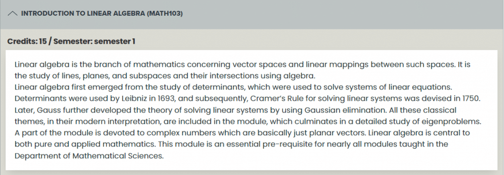
微积分代写|CALCULUS II MATH102 University of Liverpool Assignment

0

Assignment-daixieTM为您提供利物浦大学University of Liverpool CALCULUS II MATH102微积分代写代考辅导服务!

Instructions:

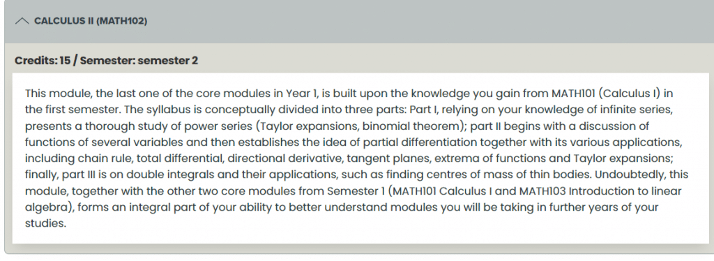
Part I of the module focuses on power series and their applications. Power series are infinite series that can represent functions as a sum of powers of a variable. You will learn about the properties of power series and their convergence, as well as the relationship between power series and functions, including how to use Taylor and Maclaurin series to approximate functions.

Part II of the module introduces functions of several variables and partial differentiation. You will learn how to find partial derivatives, including the chain rule, total differential, directional derivative, and tangent planes. Additionally, you will learn how to find extrema of functions of several variables and how to use Taylor expansions to approximate functions.

Finally, part III of the module focuses on double integrals and their applications. You will learn how to evaluate double integrals using different methods, including iterated integrals and change of variables. You will also learn how to use double integrals to find areas, volumes, and centroids of two-dimensional and three-dimensional objects.

Overall, this module, together with MATH101 and MATH103, provides a strong foundation in calculus and linear algebra, which is essential for further studies in mathematics and many other fields, such as physics, engineering, and economics.

微积分代写|CALCULUS II MATH102 University of Liverpool Assignment

问题 1.

$\vec{R} \cdot \vec{V}=0$, so $\frac{d}{d t}(\vec{R} \cdot \vec{V})=\vec{V} \cdot \vec{V}+\vec{R} \cdot \vec{A}=0$. Therefore $\vec{R} \cdot \vec{A}=-|\vec{V}|^2$.

证明 .

We can start by differentiating the expression $\vec{R} \cdot \vec{V}$ with respect to time $t$ using the product rule:

$$\frac{d}{dt}(\vec{R} \cdot \vec{V}) = \frac{d \vec{R}}{dt} \cdot \vec{V} + \vec{R} \cdot \frac{d \vec{V}}{dt}$$

Since $\vec{R} \cdot \vec{V}$ is a scalar quantity, its derivative must be a scalar as well. We can simplify the above expression using the fact that $\vec{R}$ and $\vec{V}$ are perpendicular (i.e. $\vec{R} \cdot \vec{V} = 0$), which implies that $\frac{d \vec{R}}{dt} \cdot \vec{V} = 0$. Therefore:

$$\frac{d}{dt}(\vec{R} \cdot \vec{V}) = \vec{R} \cdot \frac{d \vec{V}}{dt}$$

Now, we can substitute the expression for the acceleration $\vec{A} = \frac{d \vec{V}}{dt}$:

$$\frac{d}{dt}(\vec{R} \cdot \vec{V}) = \vec{R} \cdot \vec{A}$$

Using the chain rule, we can rewrite the left-hand side as:

$$\frac{d}{dt}(\vec{R} \cdot \vec{V}) = \frac{d\vec{R}}{dt} \cdot \vec{V} + \vec{R} \cdot \frac{d\vec{V}}{dt} = \vec{V} \cdot \vec{V} + \vec{R} \cdot \vec{A}$$

Substituting this into the previous expression, we get:

$$\vec{V} \cdot \vec{V} + \vec{R} \cdot \vec{A} = 0$$

Solving for $\vec{R} \cdot \vec{A}$, we get:

$$\vec{R} \cdot \vec{A} = -|\vec{V}|^2$$

Therefore, we have shown that $\vec{R} \cdot \vec{A} = -|\vec{V}|^2$ given the initial condition $\vec{R} \cdot \vec{V} = 0$.

问题 2.

a) $P=(1,0,0), Q=(0,2,0)$ and $R=(0,0,3)$. Therefore $\overrightarrow{Q P}=\hat{\boldsymbol{\imath}}-2 \hat{\boldsymbol{\jmath}}$ and $\overrightarrow{Q R}=-2 \hat{\boldsymbol{\jmath}}+3 \hat{\boldsymbol{k}}$.

证明 .

To calculate the vector $\overrightarrow{QP}$, we subtract the coordinates of $P$ from the coordinates of $Q$:

$$\overrightarrow{QP} = \begin{pmatrix}0-1 \ 2-0 \ 0-0\end{pmatrix} = \begin{pmatrix}-1 \ 2 \ 0\end{pmatrix} = -1\hat{\boldsymbol{\imath}} + 2\hat{\boldsymbol{\jmath}}$$

To calculate the vector $\overrightarrow{QR}$, we subtract the coordinates of $R$ from the coordinates of $Q$:

$$\overrightarrow{QR} = \begin{pmatrix}0-0 \ 2-0 \ 3-0\end{pmatrix} = \begin{pmatrix}0 \ 2 \ 3\end{pmatrix} = 2\hat{\boldsymbol{\jmath}} + 3\hat{\boldsymbol{k}}$$

So, as you said, $\overrightarrow{QP} = \hat{\boldsymbol{\imath}} – 2 \hat{\boldsymbol{\jmath}}$ and $\overrightarrow{QR} = -2\hat{\boldsymbol{\jmath}} + 3\hat{\boldsymbol{k}}$.

问题 3.

$\vec{N} \cdot \vec{r}(t)=6$, where $\vec{N}=\langle 4,-3,-2\rangle$.

证明 .

The equation $\vec{N} \cdot \vec{r}(t)=6$ represents a plane in three-dimensional space, where $\vec{N}$ is the normal vector to the plane and $\vec{r}(t)$ is a vector pointing to any point on the plane at time $t$.

Given that $\vec{N}=\langle 4,-3,-2\rangle$, we can write the equation of the plane as:

$$4x – 3y – 2z = 6$$

where $x$, $y$, and $z$ are the coordinates of any point on the plane.

Alternatively, we can express the equation in vector form as:

$$\langle 4,-3,-2\rangle \cdot \langle x,y,z\rangle = 6$$

or

$$\langle 4,-3,-2\rangle \cdot \vec{r}(t) = 6$$

where $\vec{r}(t)=\langle x(t),y(t),z(t)\rangle$ is a vector function that describes the position of any point on the plane at time $t$.

Note that there are infinitely many points on the plane described by this equation, since the equation has three variables but only one constraint. Any point that satisfies the equation $4x – 3y – 2z = 6$ lies on the plane, and there are infinitely many such points.

这是一份2023年的利物浦大学University of Liverpool CALCULUS II MATH102代写的成功案例

微积分代写|CALCULUS I MATH101 University of Liverpool Assignment

0

Assignment-daixieTM为您提供利物浦大学University of Liverpool CALCULUS I MATH101微积分代写代考辅导服务!

Instructions:

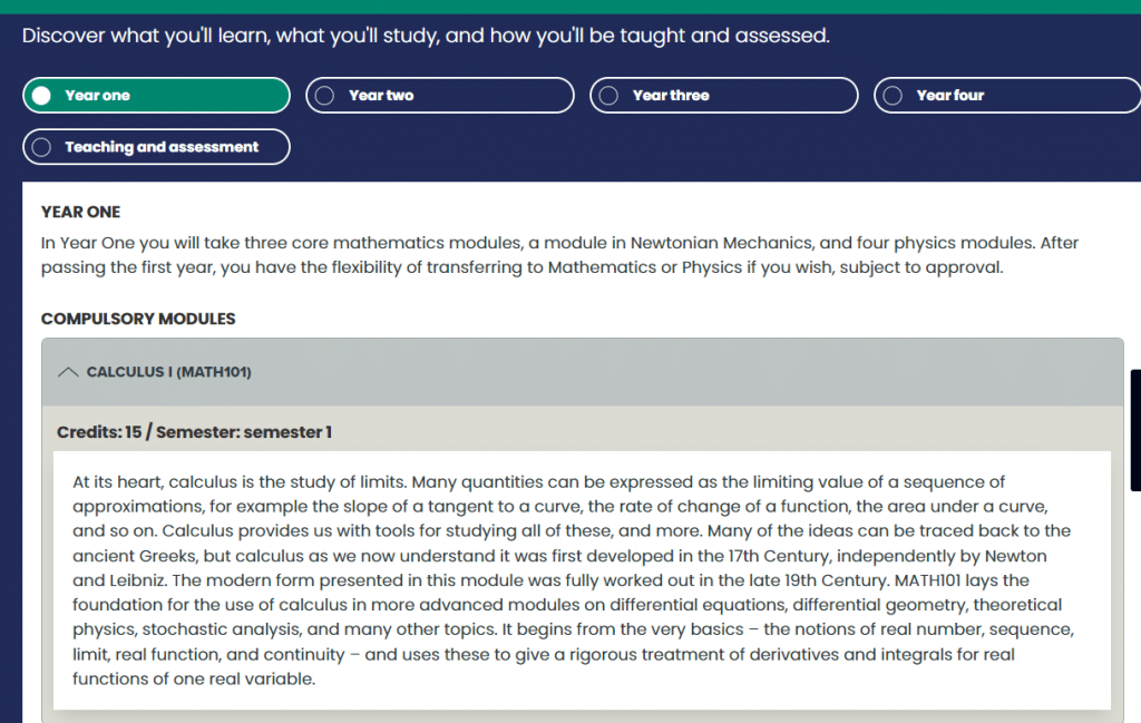
To add more details, calculus is a branch of mathematics that deals with the study of rates of change and accumulation. It is divided into two main branches: differential calculus and integral calculus.

Differential calculus deals with the study of rates of change, such as slopes of tangent lines, velocity, and acceleration. It involves concepts such as derivatives, limits, and continuity. Derivatives are used to calculate the instantaneous rate of change of a function at a specific point.

Integral calculus deals with the study of accumulation, such as finding the area under a curve or the volume of a solid. It involves concepts such as integrals, limits, and the fundamental theorem of calculus. Integrals are used to calculate the total amount of a quantity that accumulates over an interval of time or a region of space.

Calculus has numerous practical applications in various fields such as physics, engineering, economics, and biology. It provides a powerful tool for solving real-world problems by modeling them mathematically and then applying calculus techniques to obtain solutions.

微积分代写|CALCULUS I MATH101 University of Liverpool Assignment

问题 1.

$\mathrm{Q}=$ top of the ladder: $\overrightarrow{\mathrm{OQ}}=\langle 0, L \sin \theta\rangle ; \quad \mathrm{R}=$ bottom of the ladder: $\overrightarrow{\mathrm{OR}}=\langle-L \cos \theta, 0\rangle$.
Midpoint: $\overrightarrow{\mathrm{OP}}=\frac{1}{2}(\overrightarrow{\mathrm{OQ}}+\overrightarrow{\mathrm{OR}})=\left\langle-\frac{L}{2} \cos \theta, \frac{L}{2} \sin \theta\right\rangle$.
Parametric equations: $x=-\frac{L}{2} \cos \theta, y=\frac{L}{2} \sin \theta$.

证明 .

It looks like you have provided the vector representations and parametric equations for three points in a coordinate plane: point Q at the top of a ladder, point R at the bottom of the ladder, and the midpoint P between points Q and R.

The vector representation of point Q is $\overrightarrow{\mathrm{OQ}}=\langle 0, L \sin \theta\rangle$, which means that point Q is located at the origin of the coordinate plane (since the x-coordinate is 0) and has a y-coordinate of $L \sin \theta$.

The vector representation of point R is $\overrightarrow{\mathrm{OR}}=\langle-L \cos \theta, 0\rangle$, which means that point R is located on the x-axis (since the y-coordinate is 0) and has an x-coordinate of $-L \cos \theta$.

The vector representation of point P is found by taking the average of the vectors for points Q and R: $\overrightarrow{\mathrm{OP}}=\frac{1}{2}(\overrightarrow{\mathrm{OQ}}+\overrightarrow{\mathrm{OR}})=\left\langle-\frac{L}{2} \cos \theta, \frac{L}{2} \sin \theta\right\rangle$. This means that point P is located at $x=-\frac{L}{2} \cos \theta$ and $y=\frac{L}{2} \sin \theta$.

The parametric equations for these points are simply the x and y coordinates expressed as functions of the parameter $\theta$: $x=-\frac{L}{2} \cos \theta, y=\frac{L}{2} \sin \theta$. These equations allow you to plot the points on the coordinate plane as $\theta$ varies.

问题 2.

a) $\frac{d}{d t}(\vec{R} \cdot \vec{R})=\vec{V} \cdot \vec{R}+\vec{R} \cdot \vec{V}=2 \vec{R} \cdot \vec{V}$.

证明 .

We can use the product rule of differentiation and the fact that the derivative of a constant vector is zero to find the derivative of $\vec{R} \cdot \vec{R}$ with respect to time:

$$\frac{d}{dt}(\vec{R} \cdot \vec{R}) = \frac{d}{dt}(\sum_{i=1}^{n} R_i^2) = \sum_{i=1}^{n} \frac{d}{dt}(R_i^2)$$

Using the chain rule, we have:

$$\frac{d}{dt}(R_i^2) = 2R_i \frac{dR_i}{dt}$$

Therefore:

$$\frac{d}{dt}(\vec{R} \cdot \vec{R}) = \sum_{i=1}^{n} 2R_i \frac{dR_i}{dt} = 2\sum_{i=1}^{n} R_i \frac{dR_i}{dt}$$

Using the product rule of differentiation, we have:

$$\frac{d}{dt}(\vec{R} \cdot \vec{R}) = 2\sum_{i=1}^{n} R_i \frac{dR_i}{dt} = 2\sum_{i=1}^{n} R_i \frac{dR_i}{dt} + 2\sum_{i=1}^{n} R_i \frac{dR_i}{dt} = 2\sum_{i=1}^{n} R_i \frac{dR_i}{dt} + 2\sum_{i=1}^{n} \frac{dR_i}{dt} R_i$$

Using the dot product rule, we have:

$$\frac{d}{dt}(\vec{R} \cdot \vec{R}) = 2\sum_{i=1}^{n} R_i \frac{dR_i}{dt} + 2\sum_{i=1}^{n} \frac{dR_i}{dt} R_i = 2\vec{R} \cdot \vec{V}$$

Therefore, we have:

$$\frac{d}{d t}(\vec{R} \cdot \vec{R})=\vec{V} \cdot \vec{R}+\vec{R} \cdot \vec{V}=2 \vec{R} \cdot \vec{V}.$$

问题 3.

b) Assume $|\vec{R}|$ is constant: then $\frac{d}{d t}(\vec{R} \cdot \vec{R})=2 \vec{R} \cdot \vec{V}=0$, i.e. $\vec{R} \perp \vec{V}$.

证明 .

Starting with $\vec{R}\cdot\vec{R}=|\vec{R}|^2$, we can take the derivative with respect to time $t$ using the chain rule:

$$\frac{d}{d t}(\vec{R} \cdot \vec{R})=\frac{d}{d t}(|\vec{R}|^2)=2|\vec{R}|\frac{d|\vec{R}|}{dt}.$$

Since we are assuming $|\vec{R}|$ is constant, we have $\frac{d|\vec{R}|}{dt}=0$, so

$$\frac{d}{d t}(\vec{R} \cdot \vec{R})=2|\vec{R}|\frac{d|\vec{R}|}{dt}=0.$$

Therefore, $\vec{R}\cdot\vec{V}=0$ because the dot product of any two vectors is zero if and only if the vectors are perpendicular. Thus, we have $\vec{R}\perp\vec{V}$ as required.

这是一份2023年的利物浦大学University of Liverpool CALCULUS I MATH101代写的成功案例

动态系统代写|DYNAMICAL SYSTEMS MATHS4074 University of Glasgow Assignment

0

Assignment-daixieTM为您提供格拉斯哥大学University of Glasgow DYNAMICAL SYSTEMS MATHS4074动态系统代写代考辅导服务!

Instructions:

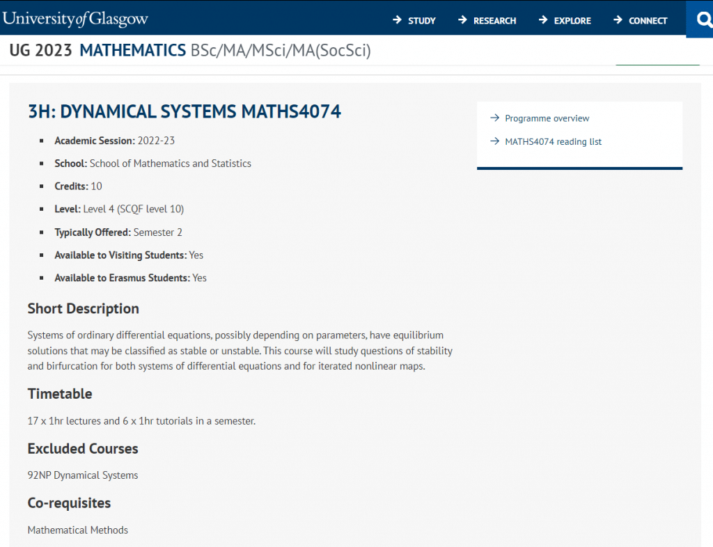
Stability analysis involves studying the behavior of solutions to differential equations or maps as time goes on. An equilibrium solution is a solution that doesn’t change over time, so it’s important to determine whether these solutions are stable (perturbations from the equilibrium decay over time) or unstable (perturbations grow over time). Depending on the system and the equilibrium solution, there are different methods for determining stability, including linearization, Lyapunov functions, and phase portraits.

Bifurcation theory is concerned with how the behavior of a dynamic system changes as parameters are varied. When a system undergoes a bifurcation, its behavior can change drastically, for example, an equilibrium solution may suddenly appear or disappear, or the system may exhibit periodic or chaotic behavior. Understanding the bifurcations that a system undergoes can provide insight into the underlying mechanisms that govern its behavior.

Overall, the topics covered in this course should provide you with a solid foundation for understanding the behavior of nonlinear systems and the methods used to analyze them.

动态系统代写|DYNAMICAL SYSTEMS MATHS4074 University of Glasgow Assignment

问题 1.

Let $A \in \mathbb{C}^{n \times n}$, and $B \in \mathbb{C}^{m \times m}$. Show that $X(t)=e^{A t} X(0) e^{B t}$ is the solution to $\dot{X}=$ $A X+X B$

证明 .

Recalling the definition of matrix exponential, $e^{A t}=\sum_{i=0}^{\infty} \frac{1}{i !}(A t)^i$, it is clear that, for any matrix $A, e^{A t}=I$ for $t=0$, and $d e^{A t} / d t=A e^{A t}=e^{A t} A$.
Hence,
$$
\begin{aligned}
\frac{d}{d t}\left(e^{A t} X(0) e^{B t}\right)=\left(\frac{d}{d t} e^{A t}\right) X(0) e^{B t}+e^{A t} & \left(\frac{d}{d t} X(0)\right) e^{B t}+e^{A t} X(0)\left(\frac{d}{d t} e^{B t}\right) \
& =A\left(e^{A t} X(0) e^{B t}\right)+0+\left(e^{A t} X(0) e^{B t}\right) B
\end{aligned}
$$
Furthermore, for $t=0$,
$$
\left.\left(e^{A t} X(0) e^{B t}\right)\right|_{t=0}=X(0)
$$
Hence we can conclude that the proposed function is in fact the solution to the initialvalue problem under consideration.

问题 2.

Use the projection theorem to solve the problem:
$$
\min _{x \in \mathbb{R}^n}\left{x^T Q x: A x=b\right}
$$
where $Q$ is a positive-definite $n \times n$ matrix, $A$ is a $m \times n$ real matrix, with rank $m<n$, and $b$ is a real $m$-dimensional vector. Is the solution unique?

证明 .

(Note that $Q$ being positive-definite implies it is self-adjoint, i.e., Hermitian.) Let $x_0$ be such that $A x_0=b$, and consider the change of variables $z=x-x_0$. In the inner product space $\mathbb{R}^n$, with inner product $\langle u, v\rangle=u^T Q v$, it is desired to minimize $|x|^2=x^T Q x=\left|z+x_0\right|^2$, subject to the constraint that $z$ lies in the subspace $M:=\left{z \in \mathbb{R}^n: A z=0\right}$. Using the projection theorem, we know that an optimal solution $\hat{z}=\hat{x}-x_0$ must be such that $\left(\hat{z}+x_0=\hat{x}\right) \perp M$, i.e., $\langle\hat{x}, y\rangle=\hat{x}^T Q y=0$, for all $y \in M$. Summarizing, we know that
$$
\begin{aligned}
\hat{x}^T Q y & =0, \quad \forall A y=0 \
A x & =b .
\end{aligned}
$$
In order to satisfy the first equation for all $y$ such that $A y=0, \hat{x}$ must be of the form $\hat{x}=Q^{-1} A^T v$, for some $v \in \mathbb{R}^m$. The vector $v$ can be found using the constraint $A x=b$, i.e.,
$$
A \hat{x}=A Q^{-1} A^T v=b,
$$
and hence
$$
v=\left(A Q^{-1} A^T\right)^{-1} b .
$$
Concluding,
$$
\hat{x}=Q^{-1} A^T\left(A Q^{-1} A^T\right)^{-1} b
$$

问题 3.

Let $|A|<1$. Show that $\left|(I-A)^{-1}\right| \geq \frac{1}{1+|A|}$.

证明 .

First of all, for any vector $x_0$, with $\left|x_0\right|=1$,
$$
\left|(I-A) x_0\right| \geq\left|x_0\right|-\left|A x_0\right| \geq 1-|A|>0
$$

which shows that the matrix $I-A$ is invertible, i.e., there is no vector $x_0$, with $\left|x_0\right|=1$, such that $(I-A) x_0=0$.
Furthermore, the following chain of inequalities holds:
$$
\begin{aligned}
1=|I|=\left|(I-A)(I-A)^{-1}\right| & \leq|I-A| \cdot\left|(I-A)^{-1}\right| \
& \leq(|I|+|A|) \cdot\left|(I-A)^{-1}\right|=(1+|A|) \cdot\left|(I-A)^{-1}\right|,
\end{aligned}
$$
and the result follows. The definition of induced norm implies that $|I|=1$. The first inequality is due to the submultiplicative property of induced norms. The second inequality can be derived from the triangle inequality.

这是一份2023年的格拉斯哥大学University of Glasgow DYNAMICAL SYSTEMS MATHS4074代写的成功案例

代数代写|ALGEBRA MATHS4072 University of Glasgow Assignment

0

Assignment-daixieTM为您提供格拉斯哥大学University of Glasgow ALGEBRA MATHS4072代数代写代考辅导服务!

Instructions:

Algebraic structures, such as groups, rings, and fields, are fundamental concepts in abstract algebra that have important applications in many areas of mathematics and beyond.

Group theory is the study of the algebraic structure called a group, which is a set of elements with a binary operation that satisfies certain axioms. Group theory has applications in many areas of mathematics, including number theory, geometry, and topology.

Ring theory is the study of rings, which are algebraic structures that generalize the properties of integers. Rings are important in algebraic geometry, number theory, and coding theory.

Field theory is the study of fields, which are algebraic structures that extend the properties of rational numbers. Fields are important in algebraic geometry, number theory, and physics.

The construction and application of quotient or factor groups and rings is an important aspect of algebraic structures. Homomorphisms between rings and groups are also essential in the study of algebraic structures.

Overall, this course will provide a solid foundation in the basic concepts and techniques of abstract algebra, which will be useful in many areas of mathematics and beyond.

代数代写|ALGEBRA MATHS4072 University of Glasgow Assignment

问题 1.

Let $[n]$ denote the totally ordered set $\{0,1, \ldots, n\}$. Let $\phi:[m] \rightarrow[n]$ be an order preserving function (so that if $i \leq j$ then $\phi(i) \leq \phi(j)$ ). Identifying the elements of $[n]$ with the vertices of the standard simplex $\Delta^n, \phi$ extends to an affine $\operatorname{map} \Delta^m \rightarrow \Delta^n$ that we also denote by $\phi$. Give a formula for this map in terms of barycentric coordinates: If $\phi\left(s_0, \ldots, s_m\right)=\left(t_0, \ldots, t_n\right)$, what is $t_j$ as a function of $\left(s_0, \ldots, s_m\right) ?$

证明 .

Let $\Delta^n$ be the standard $n$-simplex, that is, $\Delta^n = {(x_0, x_1, \ldots, x_n) \in \mathbb{R}^{n+1} : x_i \geq 0, \sum_{i=0}^n x_i = 1}$. We will use the barycentric coordinates for the points in $\Delta^n$, which are defined as follows: for $0 \leq i \leq n$, let $e_i \in \Delta^n$ be the point with $x_i = 1$ and $x_j = 0$ for $j \neq i$. Then any point $p \in \Delta^n$ can be written uniquely as a convex combination of the $e_i$’s, that is, $p = \sum_{i=0}^n \lambda_i e_i$, where $\lambda_i \geq 0$ and $\sum_{i=0}^n \lambda_i = 1$.

Now let $\phi: [m] \to [n]$ be an order-preserving function, and let $\phi:\Delta^m \to \Delta^n$ be the affine map that extends $\phi$ to the standard simplices. We want to express $\phi(p)$ in terms of the barycentric coordinates of $p = \sum_{i=0}^m \lambda_i e_i$.

Note that $\phi(e_i)$ is a point in $\Delta^n$, so we can write $\phi(e_i)$ as a convex combination of the $e_j$’s. Let $\phi(e_i) = \sum_{j=0}^n a_{ij} e_j$, where $a_{ij} \geq 0$ and $\sum_{j=0}^n a_{ij} = 1$. Then for any $p \in \Delta^m$, we have \begin{align*} \phi(p) &= \phi\left(\sum_{i=0}^m \lambda_i e_i\right) \ &= \sum_{i=0}^m \lambda_i \phi(e_i) \ &= \sum_{i=0}^m \lambda_i \sum_{j=0}^n a_{ij} e_j \ &= \sum_{j=0}^n \left(\sum_{i=0}^m \lambda_i a_{ij}\right) e_j. \end{align*}

Let $t_j = \sum_{i=0}^m \lambda_i a_{ij}$, so we have $\phi(p) = \sum_{j=0}^n t_j e_j$. Since $e_j$ is the point with $x_j = 1$ and $x_i = 0$ for $i \neq j$, we have $t_j = \phi(\lambda_j)$, where $\lambda_j$ is the $j$th barycentric coordinate of $p$. Therefore, we have

$t_j=\sum_{i=0}^m \lambda_i a_{i j}$,

where $a_{ij}$ is the $j$th barycentric coordinate of $\phi(e_i)$.

问题 2.

(a) Write $\pi_0(X)$ for the set of path-components of a space $X$. Construct an isomorphism $$ \mathbb{Z} \pi_0(X) \rightarrow H_0(X) $$

证明 .

Let $X$ be a topological space. We denote by $\pi_0(X)$ the set of path-components of $X$. That is, for any two points $x,y\in X$, we say that $x$ and $y$ are in the same path-component if there exists a path $\gamma:[0,1]\to X$ such that $\gamma(0)=x$ and $\gamma(1)=y$. The set $\pi_0(X)$ is a partition of $X$ into disjoint subsets, and each subset is a path-connected subspace of $X$.

Now, we construct an isomorphism between $\mathbb{Z} \pi_0(X)$ and $H_0(X)$. Let $\mathbb{Z}\pi_0(X)$ be the free abelian group generated by the set $\pi_0(X)$, and let $\phi:\mathbb{Z}\pi_0(X)\to H_0(X)$ be the homomorphism defined as follows. For each path-component $[x]\in \pi_0(X)$, choose a point $x\in [x]$, and define $\phi([x])=[x]$ to be the class in $H_0(X)$ represented by the point $x$. We extend $\phi$ to all of $\mathbb{Z}\pi_0(X)$ by linearity.

We claim that $\phi$ is an isomorphism. To see this, we construct its inverse. Let $\psi:H_0(X)\to \mathbb{Z}\pi_0(X)$ be the homomorphism defined by sending each class $[x]\in H_0(X)$ to the generator $[x]\in \mathbb{Z}\pi_0(X)$ corresponding to the path-component containing $x$. That is, if $[x]\in H_0(X)$, then there exists a chain $\sum_i n_i \sigma_i$ with $\sigma_i:\Delta^0\to X$ such that $\partial (\sum_i n_i \sigma_i)=[x]$, and we define $\psi([x])=[\sigma_i(0)]\in \mathbb{Z}\pi_0(X)$. Again, we extend $\psi$ to all of $H_0(X)$ by linearity.

It is easy to see that $\psi$ is well-defined and that $\phi$ and $\psi$ are inverses of each other, so $\phi$ is an isomorphism.

问题 3.

Let $A$ be a chain complex (of abelian groups). It is acyclic if $H(A)=0$, and contractible if it is chain-homotopy-equivalent to the trivial chain complex. Prove that a chain complex is contractible if and only if it is acyclic and for every $n$ the inclusion $Z_n A \hookrightarrow A_n$ is a split monomorphism of abelian groups.

证明 .

First, let’s assume that the chain complex $A$ is contractible. This means that there exists a chain map $s:A\rightarrow A$ (called a homotopy) such that $ds+sd=\mathrm{id}_A$, where $d$ is the differential of $A$. We can then define a chain map $r:A\rightarrow A$ by $r_n = \frac{1}{2}(1+s)$, which is well-defined because $s$ is a chain map. It’s easy to check that $r$ is also a chain map, and that $sr=\mathrm{id}_A$. This shows that $A$ is chain-homotopy-equivalent to the trivial chain complex.

Next, let’s assume that $A$ is acyclic and that the inclusion $Z_n A\hookrightarrow A_n$ is a split monomorphism for every $n$. Since $A$ is acyclic, we have $H_n(A)=0$ for all $n$. It remains to show that $A$ is chain-homotopy-equivalent to the trivial chain complex.

For each $n$, let $s_n:A_n\rightarrow A_{n+1}$ be a map such that $ds_n+s_{n-1}d=\mathrm{id}{A_n}$ (recall that we set $s{-1}=0$). Such a map exists because the inclusion $Z_n A\hookrightarrow A_n$ is a split monomorphism. In fact, we can take $s_n$ to be the composite of the projection $A_{n+1}\rightarrow Z_{n+1}A$ (which exists because of the split monomorphism) and the inclusion $Z_{n+1}A\hookrightarrow A_{n+1}$.

We claim that $s={s_n}$ is a chain homotopy between $A$ and the trivial chain complex. To see this, we need to show that $ds+sd=\mathrm{id}A$. We have: \begin{align*} (ds+sd)n &= d_ns{n-1}+s{n-1}d_n \ &= (s_{n-1}d-d_{n-1}s_n)+s_{n-1}d_n \ &= s_{n-1}(d_n+d_{n-1}) \ &= s_{n-1}^2 \ &= \frac{1}{4}(1+s_{n-1})^2 \ &= \frac{1}{4}(1+2s_{n-1}+s_{n-1}^2) \ &= \frac{1}{4}(1+2s_{n-1}+(1+s_{n-2})s_n) \ &= \frac{1}{4}(2s_n+s_{n-1}s_n+s_{n-2}s_n) \ &= \frac{1}{4}(2s_n+s_{n-1}d_n+s_{n-2}d_{n-1}) \ &= \frac{1}{4}(2s_n+d_{n-1}s_n+d_ns_{n-1}) \ &= \frac{1}{4}(2s_n+d_ns_{n-1}+s_{n-1}d_n) \ &= \frac{1}{4}(2s_n+\mathrm{id}{A_n}) \ &= r_n, \end{align*}

这是一份2023年的格拉斯哥大学University of GlasgowALGEBRA MATHS4072代写的成功案例

复分析代写|METHODS IN COMPLEX ANALYSIS MATHS4076 University of Glasgow Assignment

0

Assignment-daixieTM为您提供格拉斯哥大学University of Glasgow METHODS IN COMPLEX ANALYSIS MATHS4076复分析代写代考辅导服务!

Instructions:

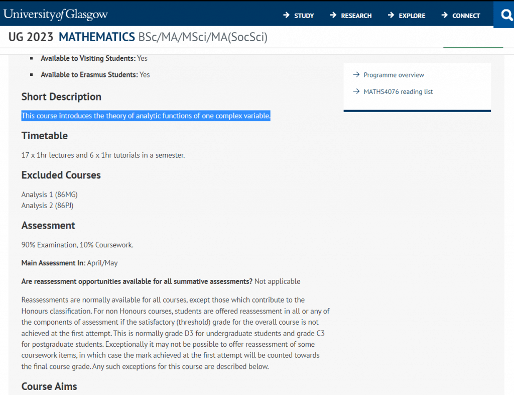
It deals with functions that are differentiable in the complex sense, meaning that they satisfy the Cauchy-Riemann equations. These functions are also called holomorphic functions.

The theory of analytic functions has many important applications in various fields, including physics, engineering, and mathematics. Some of the key topics that you might encounter in this course include power series expansions, Laurent series, singularities, residues, conformal mappings, and the Cauchy integral formula.

Throughout the course, you will learn about the properties and behavior of analytic functions, and you will develop techniques for analyzing and manipulating these functions. You will also study the connections between analytic functions and other areas of mathematics, such as complex geometry and number theory.

Overall, the study of analytic functions is a fascinating and important topic in mathematics, and it is essential for anyone interested in pursuing a career in pure or applied mathematics.

复分析代写|METHODS IN COMPLEX ANALYSIS MATHS4076 University of Glasgow Assignment

问题 1.

Let $\sum_{n=1}^{\infty} z_n$ be a convergent series of complex numbers. (1) Let $\alpha<\pi / 2$. Show that if for all $n,\left|\operatorname{Arg} z_n\right|<\alpha$, then the series $\sum_{n=1}^{\infty} z_n$ converges absolutely.

证明 . (1) Let $a_n = |z_n|$ for all $n$. Since $|\operatorname{Arg} z_n| < \alpha < \frac{\pi}{2}$, we have $\cos(\operatorname{Arg} z_n) > 0$ for all $n$. Hence, we have $$a_n = |z_n| = |z_n|\cos(\operatorname{Arg} z_n) < |z_n| \cos \alpha$$ By the comparison test, the series $\sum_{n=1}^\infty a_n$ converges. Therefore, by the absolute convergence test, the series $\sum_{n=1}^\infty z_n$ converges absolutely.

问题 2.

(2) Does the conclusion of the previous part hold if $\alpha=\pi / 2$ ?

证明 .

(2) The conclusion of part (1) does not hold if $\alpha = \frac{\pi}{2}$. For example, consider the series $\sum_{n=1}^\infty \frac{i^n}{n}$, where $i = \sqrt{-1}$. For all $n$, we have $|\operatorname{Arg} (i^n/n)| = \frac{\pi}{2}$. However, the series converges conditionally by the alternating series test.

问题 3.

(3) Assume that for all $n, \Re z_n \geq 0$ and that the series $\sum_{n=1}^{\infty} z_n^2$ also converges. Show that the series $\sum_{n=1}^{\infty} z_n^2$ converges absolutely.

证明 .

(3) Since $\Re z_n \geq 0$ for all $n$, we have $|z_n| = \sqrt{z_n \overline{z_n}} = \sqrt{z_n^2} = z_n$. Therefore, we have $$|z_n^2| = |z_n|^2 = z_n^2$$ Since the series $\sum_{n=1}^\infty z_n^2$ converges, we have $$\sum_{n=1}^\infty |z_n^2| = \sum_{n=1}^\infty z_n^2$$ converges, and hence the series $\sum_{n=1}^\infty z_n$ converges absolutely.

这是一份2023年的格拉斯哥大学University of Glasgow METHODS IN COMPLEX ANALYSIS MATHS4076代写的成功案例

度量空间和基本拓扑学代写|METRIC SPACE AND BASIC TOPOLOGY MATHS4077 University of Glasgow Assignment

0

Assignment-daixieTM为您提供格拉斯哥大学University of Glasgow METRIC SPACE AND BASIC TOPOLOGY MATHS4077度量空间和基本拓扑学代写代考辅导服务!

Instructions:

In a course on topology, you can expect to study the fundamental concepts of point-set topology, including sets, functions, continuity, convergence, compactness, and connectedness. You will learn how to use these concepts to prove theorems and solve problems in a variety of mathematical contexts.

The course will likely start with a review of basic set theory and logic, and then move on to the definition and properties of metric spaces. You will learn about various topological concepts and constructions, such as open sets, closed sets, neighborhoods, interior, closure, and boundary. You will study different types of convergence, such as pointwise, uniform, and Hausdorff convergence, and learn how to use these concepts to prove continuity and other results.

Later on, you may also study more advanced topics in topology, such as homotopy theory, algebraic topology, and differential topology. These areas of study involve the use of topological concepts and tools to solve more sophisticated problems in mathematics and other fields.

Overall, a course in topology will provide you with a deep understanding of the fundamental concepts and methods of topology, which are essential for further study in mathematics and other areas of science and engineering.

度量空间和基本拓扑学代写|METRIC SPACE AND BASIC TOPOLOGY MATHS4077 University of Glasgow Assignment

问题 1.

Consider the function $f: \mathbb{R} \rightarrow \mathbb{R}$ given by $f(x)=k x+b$ for $0<k<1$ and $b \in \mathbb{R}$. Show that $f$ is a contraction, find the fixed point of $f$, and directly show the fixed point is unique.

证明 .

To show that $f$ is a contraction, we need to show that there exists a constant $0 \leqslant L < 1$ such that for all $x, y \in \mathbb{R}$, we have $|f(x) – f(y)| \leqslant L|x-y|$.

So let $x, y \in \mathbb{R}$ be arbitrary, and let $L = k$. Then we have

\begin{align*} |f(x) – f(y)| &= |kx + b – ky – b| \ &= |k(x-y)| \ &= k|x-y|. \end{align*}

Since $0<k<1$, we have $0\leqslant L<k<1$. Therefore, $f$ is a contraction.

To find the fixed point of $f$, we need to solve the equation $f(x) = x$. That is,

$$kx+b=x$$

which gives $x = \frac{b}{1-k}$. Therefore, the fixed point of $f$ is $\frac{b}{1-k}$.

To show that the fixed point is unique, we need to show that if $x_1$ and $x_2$ are both fixed points of $f$, then $x_1 = x_2$.

So let $x_1$ and $x_2$ be fixed points of $f$. Then we have

\begin{align*} f(x_1) &= x_1 \ f(x_2) &= x_2 \end{align*}

Subtracting these equations, we get

\begin{align*} f(x_1) – f(x_2) &= x_1 – x_2 \ kx_1 + b – kx_2 – b &= x_1 – x_2 \ k(x_1 – x_2) &= x_1 – x_2 \ \end{align*}

Since $k < 1$, we can divide both sides by $k(x_1 – x_2)$ to obtain $1 < \frac{1}{k}$, which means $x_1 = x_2$. Therefore, the fixed point of $f$ is unique.

问题 2.

In class, we have defined a set $A \subset X$ to be closed if its complement is an open set in $X$. There is another useful definition of a closed set however. Show that $A \subset X$ is closed if and only if every convergent sequence in $A$ converges in $A$. In other words, if $\left\{x_n\right\}$ is a convergent sequence in $A$ such that $x_n \rightarrow x$, then $x \in A$.

证明 .

To prove that $A \subset X$ is closed if and only if every convergent sequence in $A$ converges in $A$, we need to show two things:

$(\Rightarrow)$ If $A$ is closed, then every convergent sequence in $A$ converges in $A$. $(\Leftarrow)$ If every convergent sequence in $A$ converges in $A$, then $A$ is closed.

$(\Rightarrow)$ Suppose that $A$ is closed, and let $\left{x_n\right}$ be a convergent sequence in $A$ that converges to some $x \in X$. We want to show that $x \in A$. Since $\left{x_n\right}$ converges to $x$, we know that for any open set $U$ containing $x$, there exists an $N$ such that $x_n \in U$ for all $n \geq N$. In particular, for the open set $U = X \setminus A$, we have $x_n \notin U$ for all $n \geq N$, since $\left{x_n\right}$ is a sequence in $A$. Therefore, $x \notin U$, which implies that $x \in A$ (since $U = X \setminus A$ is closed). Thus, every convergent sequence in $A$ converges to a point in $A$, as required.

$(\Leftarrow)$ Suppose that every convergent sequence in $A$ converges in $A$, and let $U = X \setminus A$. We want to show that $U$ is open. Let $x \in U$ be arbitrary. Since $x \notin A$, there exists a sequence $\left{x_n\right}$ in $A$ that converges to $x$. But by assumption, this means that $x \in A$, which is a contradiction. Therefore, $U$ contains no points of $A$, and is therefore disjoint from $A$. Thus, $U$ is open, and $A$ is closed.

Therefore, we have shown that $A$ is closed if and only if every convergent sequence in $A$ converges in $A$.

问题 3.

Let $|\cdot|$ be a norm on a vector space $V$, and let $d(x, y)=|x-y|$ for all $x, y \in V$. Show the following three properties:
(a) $d(\lambda x, \lambda y)=|\lambda| d(x, y)$ for all $\lambda \in \mathbb{R}$, and for all $x, y \in V$.

证明 .

To show that $d(\lambda x, \lambda y) = |\lambda| d(x, y)$ for all $\lambda \in \mathbb{R}$, and for all $x, y \in V$, we need to use the properties of the norm $|\cdot|$.

First, note that by the definition of $d$, we have:

$d(\lambda x, \lambda y)=|\lambda x-\lambda y|$

Using the properties of the norm, we can manipulate this expression as follows:

\begin{align*} |\lambda x – \lambda y| &= |\lambda (x – y)| \ &= |\lambda| |x – y| \ &= |\lambda| d(x, y). \end{align*}

Therefore, we have shown that $d(\lambda x, \lambda y) = |\lambda| d(x, y)$ for all $\lambda \in \mathbb{R}$, and for all $x, y \in V$. This property is known as homogeneity or scaling property of the norm.

这是一份2023年的格拉斯哥大学University of Glasgow METRIC SPACE AND BASIC TOPOLOGY MATHS4077代写的成功案例

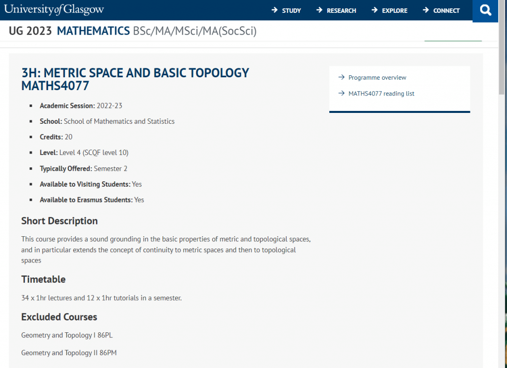
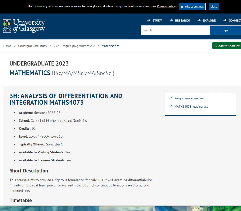
分化和整合的分析代写|ANALYSIS OF DIFFERENTIATION AND INTEGRATION MATHS4073 University of Glasgow Assignment

0

Assignment-daixieTM为您提供格拉斯哥大学University of Glasgow ANALYSIS OF DIFFERENTIATION AND INTEGRATION MATHS4073分化和整合的分析代写代考辅导服务!

Instructions:

Differentiation and integration are two fundamental operations in calculus, which is a branch of mathematics that deals with continuous change and motion. Differentiation is the process of finding the derivative of a function, while integration is the process of finding the antiderivative of a function.

Differentiation:

The derivative of a function is the rate at which the function changes with respect to its input variable. It is defined as the limit of the difference quotient as the change in the input variable approaches zero. In simpler terms, it measures how much the output of the function changes when the input changes a little bit. The derivative is denoted by the symbol “dy/dx” or “f'(x)”.

Differentiation has a number of applications, such as determining the slope of a curve at a particular point, finding the velocity and acceleration of an object, and optimizing functions in optimization problems.

分化和整合的分析代写|ANALYSIS OF DIFFERENTIATION AND INTEGRATION MATHS4073 University of Glasgow Assignment

问题 1.

Solve the initial value problem
$$
y^{\prime} y^{\prime \prime}-t=0, \quad y(1)=2, \quad y^{\prime}(1)=1 .
$$

证明 .

To solve this second-order differential equation, we first need to rewrite it as a first-order system. Let $y_1 = y$ and $y_2 = y’$, then we have:

\begin{align*} y_1′ &= y_2 \ y_2′ &= \frac{t}{y_2} \end{align*}

This gives us a first-order system that we can solve using standard techniques. To find the solution, we can use an integrating factor for the second equation. Multiplying both sides by $y_2$ gives:

y_2 y_2^{\prime}=t

We can then integrate both sides with respect to $t$ to get:

$\frac{1}{2} y_2^2=\frac{1}{2} t^2+C_1$

where $C_1$ is an arbitrary constant of integration. Solving for $y_2$, we get:

$y_2= \pm \sqrt{t^2+2 C_1}$

Using the initial condition $y'(1) = 1$, we have:

$y_2(1)= \pm \sqrt{1+2 C_1}=1$

Since $y_2$ must be positive, we can choose the positive sign and solve for $C_1$:

$\sqrt{1+2 C_1}=1 \quad \Rightarrow \quad C_1=0$

Thus, we have:

$y_2=\sqrt{t^2}=t$

Next, we can integrate the first equation:

$y_1=\int y_2 d t=\frac{1}{2} t^2+C_2$

Using the initial condition $y(1) = 2$, we have:

$y_1(1)=\frac{1}{2}+C_2=2 \quad \Rightarrow \quad C_2=\frac{3}{2}$

Thus, the solution to the initial value problem is:

$y(t)=\frac{1}{2} t^2+\frac{3}{2}$

问题 2.

Consider the differential equation $y^{\prime}=y(5-y)(y-4)^2$. (a) Determine the critical points (stationary solutions).

证明 .

(a) To find the critical points, we need to solve the equation $y^{\prime}=0$, which is equivalent to $y(5-y)(y-4)^2=0$. Therefore, the critical points are $y=0, y=5, y=4$.

问题 3.

(b)Sketch the graph of $f(y)=y(5-y)(y-4)^2$.

证明 .

(b) To sketch the graph of $f(y)=y(5-y)(y-4)^2$, we need to analyze the behavior of the function around the critical points and at infinity.

First, we can determine the sign of $f(y)$ on different intervals using test points:

\begin{array}{c|c|c|c|c} y & (-\infty,0) & (0,4) & (4,5) & (5,\infty) \ \hline y-2 & – & – & + & + \ y-3 & – & – & – & + \ y-4 & – & 0 & + & + \ y-6 & – & – & – & – \end{array}

From this table, we can see that $f(y)$ is positive on $(0,4)$ and $(5,\infty)$, and negative on $(-\infty,0)$ and $(4,5)$. Also, $f(y)$ has a local maximum at $y=4$ and local minima at $y=0$ and $y=5$.

Based on this information, we can sketch the graph of $f(y)$ as follows:

  • The function is negative and decreasing on $(-\infty,0)$.
  • The function has a local minimum at $y=0$ and increases from negative infinity to zero.
  • The function is negative and decreasing on $(0,4)$.
  • The function has a local maximum at $y=4$ and decreases from zero to the minimum value at $y=4$.
  • The function is positive and increasing on $(4,5)$.
  • The function has a local minimum at $y=5$ and increases from the minimum value at $y=5$ to positive infinity.
  • The function is positive and increasing on $(5,\infty)$.

这是一份2023年的格拉斯哥大学University of GlasgowANALYSIS OF DIFFERENTIATION AND INTEGRATION MATHS4073代写的成功案例